Linear ODEs as state-space systems
Continuous-time linear systems, the matrix exponential as fundamental solution, the damped oscillator as canonical example, and the eigenvalue classification of phase portraits.
Linear ODEs as state-space systems
1.1 What is a state-space system?
A linear state-space system is the pair of equations
where is the state at time , is the input signal, is the output, and the four matrices are real-valued with shapes , , , . The first equation is the state equation — a first-order linear ODE describing how the state evolves. The second is the output equation — a static linear readout. The integer is the state dimension; it controls how much history the model can carry forward.
The pair is “linear” because both equations are linear in and separately. It is “state-space” because summarizes everything the system needs from the past in order to predict the future given future inputs — a property called the Markov property of state. Given the present state and the input from now onward, the system’s entire future is determined.
A few conventions before going further. We treat as a column vector and apply on the left: , not . We absorb the feedthrough term into the output equation only — it appears nowhere in the state dynamics — and we will often set in examples to keep notation light. When the input is absent (), the state equation reduces to
the homogeneous linear ODE, whose solution is the focus of §1.2.
Why this object
Three reasons the state-space form is the right starting point for a book on sequence-model architectures:
- It separates dynamics from input. Whatever the input signal looks like, the dynamics matrix alone determines the system’s long-run behavior — its stability, oscillation frequencies, and decay rates. Most of the analysis in Chapter 2 looks only at .
- It generalizes immediately. Replacing the scalar derivative with a finite difference yields a discrete recurrence (Chapter 4); replacing with admits oscillatory modes (Chapter 6, Chapter 10); replacing the constant with an input-dependent yields the selective-SSM family (Chapter 9). Each generalization preserves the state-space skeleton.
- It’s the form in which continuous-time models are discretized. Every SSM derivation in the literature starts from a continuous state equation and applies a numerical integration scheme to get a discrete recurrence. If you don’t know the continuous object, the discrete one is opaque.
1.2 The matrix exponential and fundamental solutions
The homogeneous ODE with initial condition has a unique solution for every — and that solution is
where is the matrix exponential of , defined by the same series as the scalar exponential:
For any square matrix , the matrix exponential is
The series converges absolutely for every (the entrywise -norm of the partial sums is bounded by ), so is always well-defined.
The fundamental solution property — that solves the homogeneous ODE — is verified by differentiating the series term-by-term and using . The resulting derivative is , which matches . Existence and uniqueness for the inhomogeneous case () follow the variation of parameters formula
an integral that recurs (in discretized form) as the convolution kernel of every LTI SSM in Chapter 8.
Eigenvalue structure determines everything
The matrix exponential’s behavior is governed entirely by the eigenvalues of . If is diagonalizable, with , then
So acts on the eigenbasis as independent scalar exponentials. The real parts of control decay or growth: means ; means blow-up. The imaginary parts control oscillation frequency. Three regimes recur throughout the book:
- All eigenvalues with negative real part — the system is asymptotically stable: every trajectory as . This is the regime in which a recurrence “forgets” its initial state, and it is the design target for the matrices of S4, Mamba, and friends.
- At least one eigenvalue with positive real part — the system is unstable: some initial conditions blow up. A trained SSM whose drifts into this regime is the dominant numerical failure mode (Chapter 5).
- Purely imaginary eigenvalues — provided they are non-defective, the system is marginally stable and oscillates without decay; a defective imaginary eigenvalue instead picks up polynomial-in- growth and is unstable (Chapter 2 makes this precise). The non-defective modes are the energy-preserving modes of Hamiltonian systems and the natural home of symplectic discretization (Chapter 6).
When is not diagonalizable — when it has repeated eigenvalues with deficient eigenspaces — the matrix exponential picks up polynomial-in- factors on top of the terms. The Jordan normal form (Chapter 3, §3.1) gives the precise statement. For generic dense random , non-diagonalizability is a measure-zero, codimension-one event. But it is not merely pathological: it appears by design in structured systems — the critically-damped oscillator of §1.3 (a repeated real eigenvalue), and the structured/learned of HiPPO-LegS and S4 (Chapter 3). Where it occurs, those polynomial-in- factors are the whole story, not an edge case.
1.3 The damped harmonic oscillator
The canonical small example. A unit mass on a spring with stiffness and damping coefficient , displacement , evolves according to Newton’s second law,
This is a second-order scalar ODE, not first-order, so it does not yet fit the state-space template. We lift it by treating velocity as an extra state coordinate: let . Then with
This lifting trick — introduce auxiliary states to reduce ODE order to one — is the same procedure by which every higher-order ODE becomes a first-order state-space system, and it foreshadows how implicit higher-order schemes (Chapter 6) work internally.
The eigenvalues of are the roots of the characteristic polynomial :
Three sub-cases follow from the sign of the discriminant :
- Overdamped (): two real negative eigenvalues. Both modes decay monotonically; the displacement approaches zero without oscillation.
- Critically damped (): a repeated negative eigenvalue . The matrix is in this case not diagonalizable, and the solution contains a term.
- Underdamped (): a complex-conjugate eigenpair , with . Trajectories spiral toward the origin: oscillation at angular frequency with envelope decaying as .
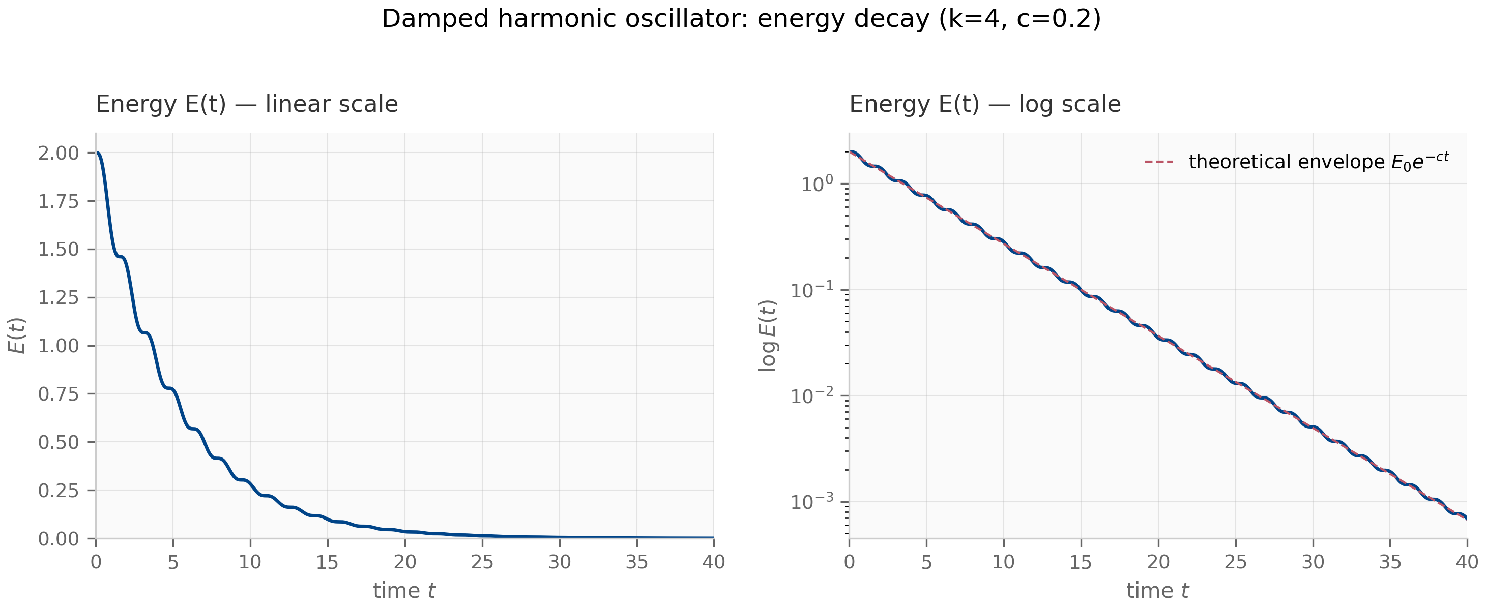
The total energy is a useful diagnostic. Its time derivative is , i.e. energy decreases monotonically whenever . Both stationary and oscillating trajectories satisfy this. The companion damped_oscillator.py simulates the underdamped regime and plots alongside the trajectory; the energy curve gives an at-a-glance check that the numerical integration preserves the dissipation structure of the continuous system.
1.4 Coupled systems and the Jacobian
The damped oscillator is a 2-dimensional toy. Real systems — and trained SSMs — live in much higher dimensions, and they typically arise from coupling many simpler subsystems. The bookkeeping is straightforward once you accept that the state vector stacks all subsystem states and encodes both intra-subsystem dynamics and inter-subsystem coupling.
A useful larger example is a ring of coupled oscillators: identical damped oscillators arranged on a circle, each coupled to its two nearest neighbors by springs of stiffness . The displacements and velocities stack into a state vector . The matrix has a block-diagonal structure for the per-oscillator dynamics, plus an off-diagonal coupling pattern that links each oscillator’s velocity equation to its neighbors’ positions:
with indices taken mod . The bracketed term is the discrete Laplacian of around the ring; it’s the same discretization of you would use in a finite-difference method for the wave equation.
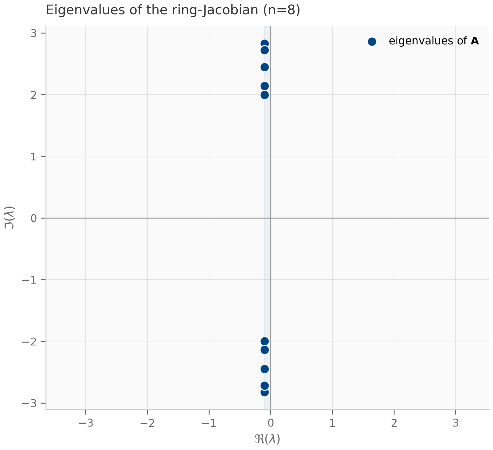
The Jacobian matrix — which for a linear system is just — has eigenvalues that are easy to compute analytically because of the ring’s circulant structure. They come in complex-conjugate pairs
(for the underdamped regime). Each indexes a standing wave mode on the ring with wavenumber ; the mode is uniform translation (no spatial structure), (when is even) is the maximally-oscillating mode where adjacent oscillators move in antiphase. The companion coupled_oscillators.py constructs for and visualizes the eigenvalues in the complex plane.
The key qualitative lesson: once you have the right state-space lift, even a system with rich spatial structure reduces to “compute eigenvalues of , classify by real and imaginary parts.” The eigenvalue distribution of a trained SSM’s — pre-training, mid-training, and converged — is one of the most informative diagnostics you can compute (Chapter 2, §2.2; Chapter 5).
The Jacobian beyond linear systems
For a nonlinear system , the Jacobian is the matrix of partial derivatives at . The linearization around a fixed point (where ) describes how small perturbations evolve. The eigenvalues of then determine local stability of by the same classification as in §1.2.
Trained recurrent networks — including SSMs in inference mode — are formally nonlinear (the state update is state = f(state, input) where f includes the input-dependent matrices). The linearization-around-a-state gives a local state-space system at each time step, and tracking how that local varies along a trajectory is the foundation of the Lyapunov-exponent analysis in Chapter 2.
1.5 Phase portraits and the eigenvalue classification
A phase portrait is the geometric picture of all trajectories of an autonomous system in state space, drawn as oriented curves. For 2-dimensional linear systems on , the topology of the portrait is determined entirely by the trace and the determinant — equivalently, by the eigenvalues — and the standard classification gives six qualitative behaviors:
| Region in -plane | Eigenvalues | Phase portrait | |---|---|---| | , , | Real negative | Stable node | | , , | Real positive | Unstable node | | , , | Complex conjugate, | Stable spiral | | , , | Complex conjugate, | Unstable spiral | | , | Pure imaginary | Center (closed orbits) | | | Real, opposite signs | Saddle |
The damped oscillator’s overdamped and underdamped sub-cases realize two of these — stable node and stable spiral — while the critically-damped case sits on the boundary as a stable degenerate node, a borderline behavior the six-way classification above does not tabulate. The undamped limit slides the eigenvalues onto the imaginary axis, turning the spiral into a center; this is the Hamiltonian limit where energy is conserved exactly.
For higher-dimensional systems the topology is richer (think: 3-D systems can have spirals around line-shaped invariant manifolds), but the building blocks are the same: each pair of complex-conjugate eigenvalues contributes a 2-D spiral subspace, each real eigenvalue contributes a 1-D direction of decay or growth. This decomposition by invariant subspaces — equivalently, by the Jordan blocks of — is the geometric content of the matrix exponential’s eigenvalue structure (§1.2).
1.6 A preview of frequency response
The variation-of-parameters formula
expresses the state as a convolution of the input with the kernel . The output (taking ) is therefore
The function for (and zero otherwise) is the impulse response of the system: the output you would observe if the input were a Dirac delta .
Taking the Laplace transform turns convolution into multiplication. With and similarly for , you get
where is the transfer function. The eigenvalues of — already shown to govern — appear as the poles of , since blows up exactly when equals an eigenvalue of . The poles’ location in the complex -plane mirrors the eigenvalue classification of §1.5: left-half-plane poles ⇔ stable system; right-half-plane poles ⇔ unstable; imaginary-axis poles ⇔ marginally stable / oscillatory.
This connection is the bridge to Chapter 8, where you’ll see that the S4 layer’s convolutional view is literally a numerical evaluation of the impulse response at uniformly spaced time points, and to Chapter 11, where the spectral structure of long convolution kernels (Hyena, RetNet) is analyzed via the same transfer-function framing.
1.7 What’s next
The next two chapters develop the analytical machinery that this chapter has only sketched. Chapter 2 makes the eigenvalue-stability story rigorous (Lyapunov, A-stability, BIBO) and adds the QR-based computational method for tracking eigenvalue trajectories during training. Chapter 3 introduces the structured-matrix vocabulary (Toeplitz, semiseparable, Vandermonde, Cauchy) needed to discuss the kernel constructions of S4 and friends. Chapters 4–6 then take the continuous state-space system here and discretize it — first crudely (ZOH, bilinear), then with full numerical-analysis machinery (Butcher tableau, A-stability), then via implicit and structure-preserving methods (Gauss–Legendre, symplectic integrators), which is where the active research pilot’s anchor (the C1 pilot) lives.
You can also profitably jump ahead: Chapter 8’s LTI SSM presentation reuses everything in this chapter and is self-contained for readers who want to see the SSM application before working through the full math foundation.
1.8 Exercises
Seven problems mixing computation and theory. Short/numerical exercises (1–4) have inline collapsible solutions; long/proof exercises (5–7) have full worked solutions in §1.9.
Exercise 1.1 (computation)
Compute the matrix exponential of by hand, term-by-term, and verify it equals the rotation matrix .
Solution
Compute powers: , so , , and the pattern repeats with period 4. Splitting the series by parity:
which expands to . ∎
Exercise 1.2 (computation)
For the damped oscillator with and , classify the damping regime and find the eigenvalues of .
Solution
Discriminant: , so the system is underdamped. Eigenvalues: . The trajectory spirals toward the origin with envelope decay rate and angular frequency .
Exercise 1.3 (computation)
Lift the third-order ODE into a 3-dimensional state-space system . Write and explicitly.
Solution
Let . Then , and from the ODE , so
The bottom row encodes the ODE’s coefficient signature; the upper-triangular ones implement the bookkeeping . This is the companion form of the ODE.
Exercise 1.4 (computation)
For the ring of identical damped oscillators with , , (no damping, symmetric coupling), use the formula in §1.4 to find the eigenvalues of analytically. Confirm they lie on the imaginary axis (since ) and verify by running companions/ch01/jax/coupled_oscillators.py with .
Solution
With , for . Numerically:
- :
- :
- :
- : same as by symmetry ⇒
All 8 eigenvalues are pure imaginary (centers), as expected for an undamped conservative system. The numerical verification reproduces these (modulo double-precision noise).
Exercise 1.5 (theory) — solution in §1.9
Prove that the matrix-exponential series converges absolutely (entrywise) for every square matrix , with bound where is the Frobenius norm.
Exercise 1.6 (theory) — solution in §1.9
Show that if is skew-symmetric (), then is orthogonal for every (that is, ). Use this to give a geometric reason why the rotation matrix of Exercise 1.1 is orthogonal.
Exercise 1.7 (theory) — solution in §1.9
Prove the variation of parameters formula: the unique solution of with is
1.9 Full solutions to theory exercises
Solution to Exercise 1.5
Let denote the Frobenius norm, which satisfies the sub-multiplicative property . Then by induction. Therefore
The partial sums are entrywise bounded by terms of a convergent scalar series, so each matrix entry is Cauchy in and converges. The limit is what we call . The bound follows by passing to the limit. ∎
Solution to Exercise 1.6
We have and . Let . Then
since by skew-symmetry. So for all , i.e. is orthogonal.
Geometric interpretation: the rotation matrix of Exercise 1.1 was generated by , which is skew-symmetric. So is orthogonal — which we already knew, but this derivation pins down why: orthogonality follows structurally from skew-symmetry of the generator, not from any property of the cos/sin functions. ∎
Solution to Exercise 1.7
Define by the formula on the right-hand side. We verify (a) the initial condition and (b) the ODE.
Initial condition. At the integral vanishes (zero-length interval) and , so . ✓
ODE. Differentiate using the product rule on the integral (Leibniz’s rule for differentiating under the integral sign):
Uniqueness follows from the classical Picard–Lindelöf theorem applied to the right-hand side , which is Lipschitz in uniformly in with constant (see Hairer–Nørsett–Wanner Hairer et al. (1993) for the standard proof). ∎
1.10 Companion code
Three JAX companions and one PyTorch companion for Chapter 1.
JAX (companions/ch01/jax/):
damped_oscillator.py— simulates the underdamped oscillator, plots energy decay (Figure 1.1)coupled_oscillators.py— constructs the ring-Laplacian state matrix, plots eigenvalue spectrum (Figure 1.2)matrix_exponential.py— comparesscipy.linalg.expmagainst truncated series sums; the truncated series catastrophically diverges for matrices with large spectral radius (auxiliary, used by Exercise 1.5)
PyTorch (companions/ch01/torch/):
matrix_exponential.py— the truncated-series-vs-torch.linalg.matrix_expcomparison, making the idiomatic-JAX vs idiomatic-PyTorch contrast concrete (compute-and-parity only; the JAX companions produce the figures).tests/— cross-framework parity: the torch partial sums and convergence curves match their JAX counterparts.
JAX companions import their plotting style from companions/_shared/plot_utils.py. To run from the repo root:
PYTHONPATH=. python companions/ch01/jax/damped_oscillator.py
PYTHONPATH=. python companions/ch01/jax/coupled_oscillators.py
PYTHONPATH=. python companions/ch01/jax/matrix_exponential.py
PYTHONPATH=. python companions/ch01/torch/matrix_exponential.pyFigures are written to public/figures/ch01/ and referenced from the <Figure> components above.
Stability theory: Lyapunov, A-stability, BIBO
Three distinct notions of stability — Lyapunov (eigenvalue criterion + QR-based computation), A-stability (regions of absolute stability for ODE integrators), and BIBO (bounded-input bounded-output for LTI systems).
Stability theory: Lyapunov, A-stability, BIBO
2.1 Three notions of stability
For the rest of this chapter, the system under analysis is the LTI state-space model from Chapter 1:
with . The three notions:
- Lyapunov stability asks: with , do trajectories stay bounded as ? Asymptotically stable if .
- A-stability is a property of a numerical integrator, not of the system. It asks: does the integrator preserve Lyapunov stability for every stable LTI test problem, at every step size ? If yes, the method is A-stable.
- BIBO stability asks: for the input–output mapping , does every bounded input () produce a bounded output? The system is BIBO-stable if yes.
When has all eigenvalues in the open left half-plane (LHP), all three coincide for the LTI case. But:
- A system can be Lyapunov-stable but not asymptotically stable (centers: pure imaginary eigenvalues, oscillations don’t decay).
- A-stability is an integrator property; the explicit Euler method is not A-stable, while the implicit Euler method is. The same continuous system therefore may need a stable integrator to preserve its stability.
- BIBO depends on the transfer function and on the choice of realization. Two systems with the same can have different BIBO properties if their “hides” unstable modes.
The rest of the chapter develops each notion in turn.
2.2 Lyapunov stability: theory
We restrict to the homogeneous case (zero input). The eigenvalue criterion is essentially the content of Chapter 1, §1.2, formalized:
Let with eigenvalues . The system is:
-
Lyapunov-stable (trajectories bounded) iff every satisfies , and for every on the imaginary axis (), its algebraic multiplicity equals its geometric multiplicity (no defective Jordan blocks).
-
Asymptotically stable (trajectories ) iff every satisfies , i.e. all eigenvalues are in the open left half-plane.
-
Unstable otherwise.
The proof reduces to the matrix-exponential formula. If is diagonalizable, then and the -th eigencomponent decays like . The Jordan-block caveat in case (1) handles the case where a defective imaginary eigenvalue produces polynomial growth in even though the real part is zero.
For nonlinear systems, the local-linearization picture from Chapter 1, §1.4 makes the same theorem applicable at each fixed point: the fixed point is asymptotically stable if the Jacobian’s eigenvalues all sit in the LHP. This is the principle that makes “check the eigenvalues” the first move in nearly every SSM stability analysis.
The Lyapunov equation
There’s an alternative characterization of asymptotic stability that doesn’t require computing eigenvalues. The continuous-time Lyapunov equation
(with a given symmetric positive-definite matrix) has a unique symmetric positive-definite solution if and only if is asymptotically stable. The function is then a Lyapunov function for the system: for all nonzero , so decreases along trajectories and forces them to the origin.
For SSM analysis, the Lyapunov-equation view is occasionally useful — for example, the controllability and observability Gramians of an LTI realization are Lyapunov solutions Antoulas (2005) — but the eigenvalue criterion is the more direct tool.
2.3 Lyapunov exponents: computation
The eigenvalues of work as a stability diagnostic for LTI systems, where is constant. For systems where the linearization varies with time (e.g. a trained recurrent network in inference mode, where the per-step Jacobian depends on the input), eigenvalues at any single don’t tell the long-run story. The right tool is the Lyapunov exponent, which generalizes the eigenvalue’s real part to time-varying systems.
Given a sequence of transition matrices (the Jacobians of an iterated map at points along a trajectory), let . The -th Lyapunov exponent is
where are the singular values of . The vector is the Lyapunov spectrum.
Three things make Lyapunov exponents the right object:
- They generalize eigenvalues to time-varying systems. For a constant Jacobian , where are the eigenvalues’ magnitudes (in the discrete case) or (in the continuous case). The connection back to Chapter 1’s eigenvalue classification is exact in the autonomous case.
- The maximal Lyapunov exponent measures sensitive dependence. A positive means infinitesimally close initial conditions diverge exponentially (chaos); is the edge-of-chaos regime; means contracting dynamics.
- They are robust to coordinate changes. Eigenvalues of the per-step Jacobian depend on the basis you write the state in; Lyapunov exponents do not.
The QR algorithm
Computing for large directly is numerically impossible: even for a well-behaved system with , after steps the largest singular value is and the smallest may be . The product matrix becomes either numerical zero or numerical infinity in finite-precision arithmetic, and finite-precision singular values lose all meaning. The fix, due to Benettin et al. Benettin et al. (1980) , is to factor the growth out at every step using QR decomposition.
The QR-based Lyapunov algorithm (the version that has become standard in dynamical-systems software):
Initialize Q_0 = I (identity), running sums L_i = 0 for i = 1..N.
For t = 1, 2, ..., T:
M_t = J_t @ Q_{t-1} # one-step forward propagation
Q_t, R_t = qr(M_t) # extract orthogonal + upper triangular
Update L_i += log |R_t[i,i]| for each i
At the end:
Lyapunov_i = L_i / TThe key insight: by re-orthonormalizing the propagated frame at every step, we factor the exponential growth into the diagonal of the upper-triangular rather than letting it accumulate in . The diagonal entries of are well-conditioned numbers near 1, and their logarithms sum nicely to give the Lyapunov exponents.
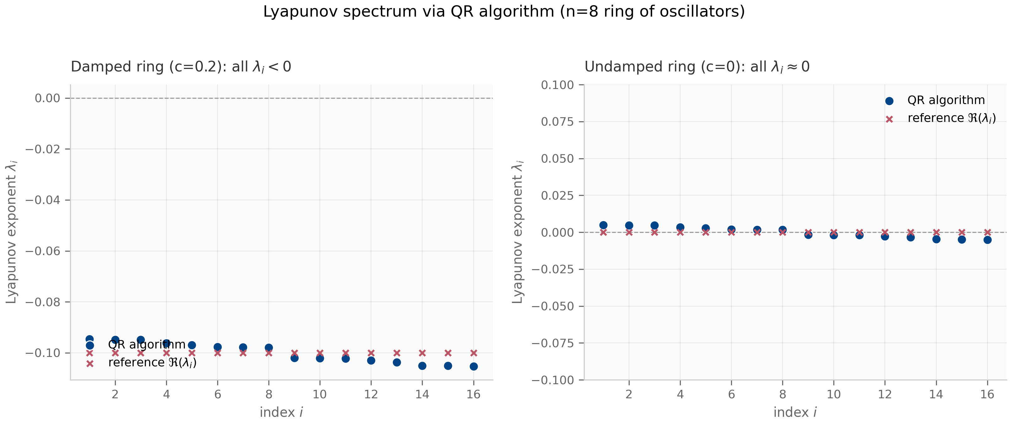
The companion lyapunov_qr.py implements this algorithm and applies it to the ring of coupled oscillators from Chapter 1, §1.4. The resulting spectrum’s structure — all exponents negative for the damped case, all near zero for the undamped case — matches the eigenvalue analysis exactly, validating the implementation.
2.4 A-stability: integrator regions of absolute stability
Switch perspectives. We now have a continuous system and we discretize it with some numerical integrator at step size . The integrator approximates the true continuous trajectory by a discrete recurrence
where is the integrator’s stability function, evaluated at the matrix argument via the matrix-functional-calculus convention. Different integrators give different :
- Forward (explicit) Euler: , so .
- Backward (implicit) Euler: , giving .
- Bilinear (Tustin / trapezoidal): .
- Exact (zero-order hold): . This is the integrator S5 and the Mamba line use by default (the original S4 used bilinear; see Chapter 8).
The discrete recurrence is Lyapunov-stable if and only if every eigenvalue of satisfies (the discrete-time analog of the LHP criterion is the unit disk). Since the eigenvalues of are where are the eigenvalues of , the question reduces to: for which in the complex plane is ?
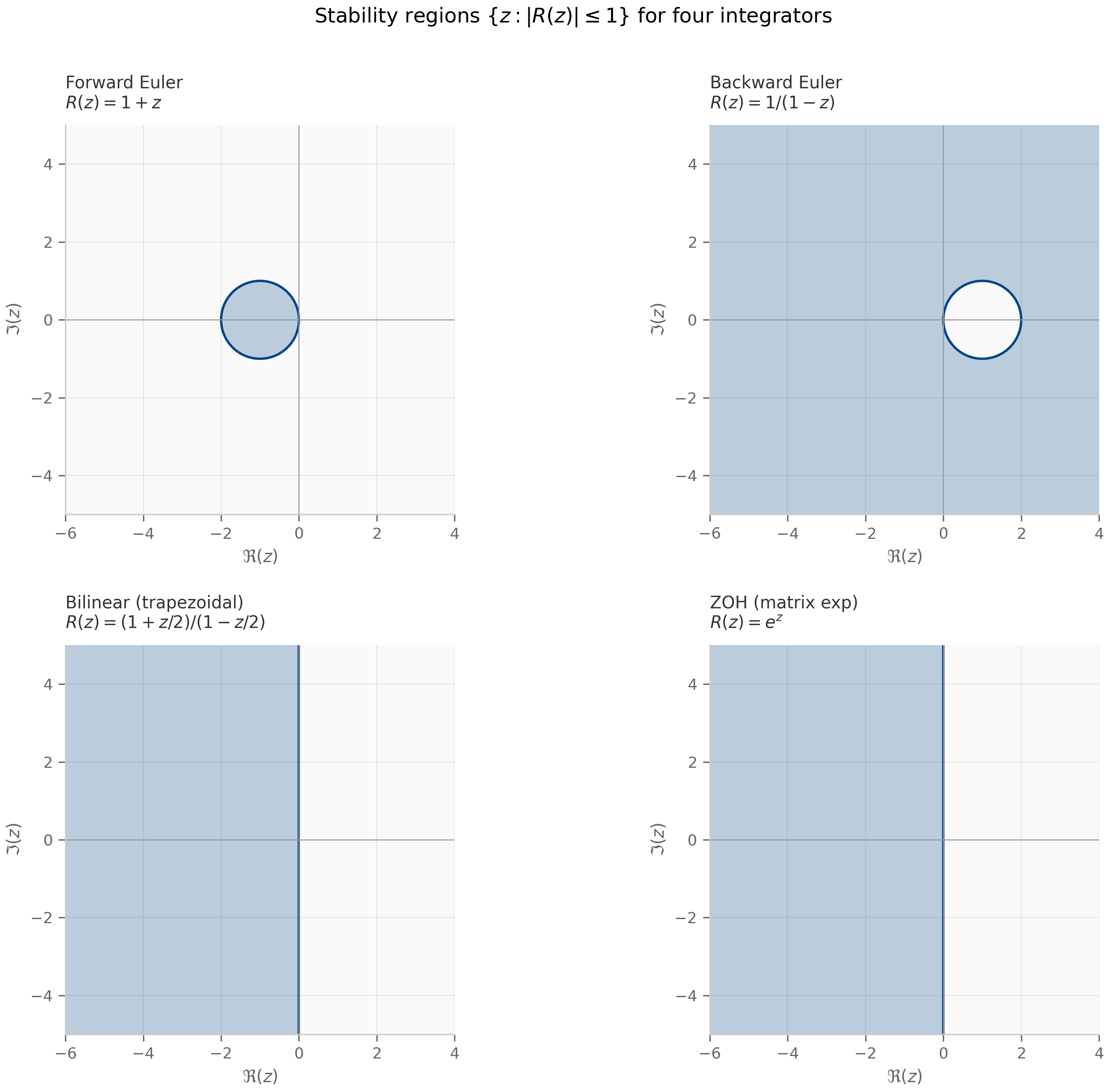
The region of absolute stability of a numerical integrator with stability function is
The integrator is A-stable if contains the entire closed left half-plane.
A-stability matters because it means: if the continuous system is asymptotically stable, the integrator preserves that stability at every step size . Without A-stability, you have to pick small enough that lands inside the (bounded) stability region.
The four examples above:
- Forward Euler: ⇔ in the closed disk of radius 1 around . Tiny region; not A-stable. For a continuous system with eigenvalue (fast decay), forward Euler requires to avoid blowup.
- Backward Euler: ⇔ ⇔ outside the open disk of radius 1 around . This contains the entire closed LHP. A-stable.
- Bilinear (trapezoidal): ⇔ exactly. The stability region is exactly the closed LHP. A-stable, and the boundary coincides with the imaginary axis — a property called L-stability when combined with as , which bilinear does not satisfy ().
- Zero-order hold (matrix exponential): ⇔ . The stability region is the closed LHP. A-stable and L-stable. This is the gold standard for LTI discretization — and it’s the scheme S5, the Mamba line, and this book’s SSM chapters standardize on.
Why this matters for SSMs
The S4 family discretizes with A-stable schemes throughout — bilinear in the original S4, ZOH in S5 — so the layer is stable at every step size for which the continuous system is stable. Mamba-1 uses ZOH as well. Mamba-3’s exponential-trapezoidal rule (Chapter 10) is a second-order generalization of bilinear that retains A-stability Lahoti et al. (2026) . The C1 research pilot (see Chapter 6) asks whether symplectic integrators — A-stable methods designed to preserve geometric invariants — can do better for complex-state SSMs whose has near-imaginary eigenvalues.
When a stability-region analysis fails, it usually fails dramatically: a forward-Euler discretization of a stiff system blows up in a handful of steps. This is exactly the failure mode that careful integrator choice prevents.
For full coverage of A-stability theory and a wider zoo of integrator stability functions, Hairer–Wanner’s stiff-systems volume Hairer & Wanner (1996) is the canonical reference.
2.5 BIBO stability
The third notion looks at the input–output mapping rather than the autonomous dynamics. For the system , , the output under a unit-impulse input is the impulse response
The system is BIBO-stable if its impulse response satisfies , equivalently if . Under this condition, any bounded input produces a bounded output — Young’s inequality on convolutions gives the precise bound .
A causal LTI system is BIBO-stable iff all poles of its transfer function lie in the open left half-plane.
Poles of are the values of where — i.e. the eigenvalues of — unless a pole–zero cancellation occurs because doesn’t “see” some eigenmode. This cancellation matters: a system can be internally unstable (some in the right half-plane) but BIBO-stable if those unstable modes are unobservable from and unreachable from . The Kalman canonical-decomposition theorem makes this precise; for our purposes, the eigenvalues of in the LHP are sufficient for both internal and BIBO stability.
For an SSM viewed as a sequence-to-sequence map, BIBO is the natural input–output stability concept: bounded inputs (typical of token embeddings) should produce bounded outputs (typical of pre-softmax logits). When training an SSM produces an whose eigenvalues drift into the right half-plane, both internal (Lyapunov) and input–output (BIBO) stability fail simultaneously, and the model’s outputs blow up. Tracking the eigenvalues of during training is therefore a single diagnostic for both failure modes.
2.6 Connection to Lyapunov functions
The Lyapunov-function method gives a non-spectral way to prove stability. For nonlinear systems where eigenvalues don’t directly apply, finding a function with , for , and for all proves asymptotic stability of .
For our LTI case , the Lyapunov equation (with p.d.) gives as a quadratic Lyapunov function — and its existence with p.d. is equivalent to asymptotic stability (as noted in §2.2). The interest in the function-method picture for our context is mainly conceptual: it explains why “energy” arguments work to prove stability of mechanical systems (the energy is the Lyapunov function), and it generalizes immediately to nonlinear systems where the eigenvalue criterion only gives local information at fixed points.
This connects forward to Chapter 6, where the question of which discretization preserves a Lyapunov function (or, more strongly, an energy invariant) leads naturally into symplectic methods.
2.7 What’s next
Chapter 3 develops the structured-linear-algebra vocabulary (SVD, Jordan form, condition number, Toeplitz/Vandermonde/Cauchy/semiseparable structure) needed for the SSM kernel constructions in Chapters 7–9. Chapter 4 takes the discretization story started in §2.4 and develops it systematically: order conditions, accuracy classes, the Butcher tableau, the bilinear and ZOH derivations in detail. Chapter 6 picks up the A-stability theme and pushes into implicit and structure-preserving integrators — symplectic schemes, geometric integration, and the C1 pilot’s home territory.
2.8 Exercises
Six problems. Inline-collapsible solutions for the shorter ones; full solutions for the longer theory problems in §2.9.
Exercise 2.1 (computation)
Use the eigenvalue criterion (Theorem 2.1) to classify the stability of for .
Solution
Characteristic polynomial: . Roots: . Both have , so the system is asymptotically stable. The non-zero imaginary part means trajectories spiral toward the origin (stable spiral).
Exercise 2.2 (computation)
For the matrix of Exercise 1.1, find the eigenvalues and classify the Lyapunov stability. Is the system asymptotically stable?
Solution
Eigenvalues: . Both have , so the system is Lyapunov-stable but not asymptotically stable — trajectories are bounded (centers / closed orbits) but do not decay to zero. This is the undamped harmonic oscillator’s marginal case.
Exercise 2.3 (computation)
The forward Euler method has stability function . For the continuous test problem with (a stiff system with fast time scale), find the maximum step size for which forward Euler is stable.
Solution
Stability condition: with . Algebra: ⇔ ⇔ . So forward Euler requires . Any produces exponentially growing iterates even though the continuous system decays. This is the classic motivation for implicit methods on stiff problems.
Exercise 2.4 (computation)
Show that the bilinear method maps the closed left half-plane onto the closed unit disk . (This is the Möbius map picture of the bilinear transform.)
Solution
Let with . Compute:
The denominator minus the numerator equals (since ). So numerator denominator and . Equality iff (purely imaginary ), so the imaginary axis maps to the unit circle and the open LHP maps to the open unit disk. ∎
Exercise 2.5 (theory) — solution in §2.9
State and prove the Lyapunov equation characterization of asymptotic stability: is asymptotically stable iff for every symmetric positive-definite , the equation has a unique symmetric positive-definite solution .
Exercise 2.6 (theory) — solution in §2.9
Prove the BIBO criterion of Theorem 2.4: a causal LTI system is BIBO-stable iff all poles of its transfer function lie in the open left half-plane. (Hint: Use the Laplace-transform / convolution duality, and exploit the representation of the impulse response as a sum of exponentials.)
2.9 Full solutions to theory exercises
Solution to Exercise 2.5
Forward direction (Lyapunov equation ⇒ asymptotic stability): Suppose is symmetric positive-definite and satisfies for some symmetric positive-definite . Define . Then for (since ), and along trajectories :
So is a strict Lyapunov function and trajectories satisfy for determined by the smallest eigenvalue of over the largest of . Hence and the origin is asymptotically stable.
Reverse direction (asymptotic stability ⇒ Lyapunov equation has p.d. solution): Suppose is asymptotically stable. Define
The integral converges absolutely because decays exponentially. is symmetric (transpose preserves the integrand structure) and positive-definite (since and is invertible). Direct computation:
using the decay of at . Uniqueness of follows from the linearity of the Lyapunov operator : its eigenvalues are the pairwise sums of eigenvalues of , so its kernel is trivial whenever no two eigenvalues sum to zero — which holds here because asymptotic stability gives for all . ∎
Solution to Exercise 2.6
(⇒) BIBO-stable implies poles in open LHP. Suppose the system is BIBO-stable, i.e. . The Laplace transform then exists and is analytic for (since the integrand is bounded by which is integrable, the integral converges uniformly). is rational (the matrix-inverse formula gives , a ratio of polynomials with denominator ). A rational function analytic on the closed right half-plane has no poles there — so all poles of lie in the open LHP.
(⇐) Poles in open LHP implies BIBO-stable. Suppose all poles of lie in the open LHP. Partial-fraction decomposition gives where are the poles with multiplicity , and for all . The inverse Laplace transform of each term is , which is on because the exponential decay beats any polynomial growth in . Sum of functions is , so and BIBO holds.
(For the multi-input multi-output case, apply the same argument entrywise to .) ∎
2.10 Companion code
Two JAX companions and one PyTorch companion for Chapter 2.
JAX (companions/ch02/jax/):
lyapunov_qr.py— implements the QR-based Lyapunov-exponent algorithm and applies it to the ring-of-oscillators system from Chapter 1stability_regions.py— plots the regions of absolute stability for forward Euler, backward Euler, bilinear (trapezoidal), and ZOH in the complex plane
PyTorch (companions/ch02/torch/):
lyapunov_qr.py— the QR-based Lyapunov spectrum in idiomatic PyTorch (thejax.lax.scan-vs-eager-loop contrast with the JAX companion; compute-and-parity only, the JAX companion produces the figure).tests/— cross-framework parity: the torch Lyapunov spectra match their JAX counterparts.
To run from the repo root:
PYTHONPATH=. python companions/ch02/jax/lyapunov_qr.py
PYTHONPATH=. python companions/ch02/jax/stability_regions.py
PYTHONPATH=. python companions/ch02/torch/lyapunov_qr.pyFigures land in public/figures/ch02/ (referenced from §2.3 and §2.4 above).
Linear algebra for sequence models: structured matrices and conditioning
Eigenvalue and SVD decompositions, condition number, the four structured-matrix families (Toeplitz, Vandermonde, Cauchy, semiseparable), low-rank updates, and a Krylov-subspace primer — the linear-algebra vocabulary later chapters assume.
Linear algebra for sequence models: structured matrices and conditioning
3.1 Eigenvalue decomposition and Jordan normal form
Chapter 1’s matrix exponential built directly on the spectral structure of . The fundamental theorem is:
For every matrix , there exist matrices (invertible) and (block-diagonal with Jordan blocks on the diagonal) such that
is the Jordan normal form of ; the diagonal entries of are the eigenvalues of (counted with algebraic multiplicity); for each eigenvalue, the number of Jordan blocks equals its geometric multiplicity and the sum of their sizes equals its algebraic multiplicity. If every eigenvalue has equal algebraic and geometric multiplicity, all Jordan blocks have size 1 and is diagonal — is diagonalizable.
A Jordan block of size for eigenvalue looks like
i.e. eigenvalue on the diagonal, ones on the superdiagonal, zeros elsewhere. The matrix exponential of a Jordan block is
which is the source of the polynomial-in- factors mentioned in Chapter 1, §1.2 — they appear exactly when there are Jordan blocks of size .
For SSM analysis, the diagonalizable case dominates. Almost every arising from random initialization or from training is diagonalizable; the non-diagonalizable case is a measure-zero, codimension-one subset of parameter space and shows up only at carefully-tuned boundaries. But structured or learned — HiPPO-LegS, S4’s DPLR parametrization, the critically-damped regime of §1.3 — can carry Jordan structure by design, and Chapter 2’s Lyapunov theorem explicitly handles the defective case.
3.2 Singular value decomposition
The eigenvalue decomposition requires to be square; for general (rectangular or possibly non-diagonalizable) matrices, the right tool is the singular value decomposition.
For every matrix , there exist orthogonal matrices , , and a diagonal-with-zeros matrix with non-negative entries on the diagonal, such that
The are the singular values of ; they are uniquely determined. The number of nonzero equals .
The SVD has three properties that make it the workhorse of numerical linear algebra:
- It always exists. Unlike the eigenvalue decomposition, no diagonalizability or even squareness assumption is needed.
- The singular values give the Frobenius and operator norms. (operator norm, equal to the largest singular value); .
- It reveals low-rank structure cleanly. Truncating the SVD at rank — keeping only the top singular values and corresponding columns of — gives the best rank- approximation to in both Frobenius and operator norms (the Eckart–Young theorem).
For square , the singular values are related to but distinct from the eigenvalues. The relationship (using descending order on both sides) lets you compute singular values via an eigenvalue problem on the Gram matrix — though in practice the QR-iteration-based SVD algorithm (LAPACK’s gesdd) is more numerically stable.
The SVD shows up explicitly in:
- Chapter 2’s Lyapunov-exponent computation (singular values of the propagated frame matrix).
- Chapter 8’s HiPPO matrix analysis (the conditioning of the projection operator is given by its SVD).
- Chapter 12’s delta-rule lineage (DeltaNet’s state update is a rank-1 SVD correction).
For a textbook treatment of the SVD’s properties and algorithms, Trefethen–Bau Trefethen & Bau (1997) Chapters 4–5 are the standard reference. Golub–Van Loan Golub & Van Loan (2013) covers the algorithmic details exhaustively.
3.3 Condition number
The condition number of a matrix (with respect to the operator norm) is
the ratio of the largest to smallest singular value (when is invertible; otherwise ). The condition number measures how much amplifies relative input perturbations into relative output perturbations: if and has relative error , then the relative error in the computed solution can be as large as .
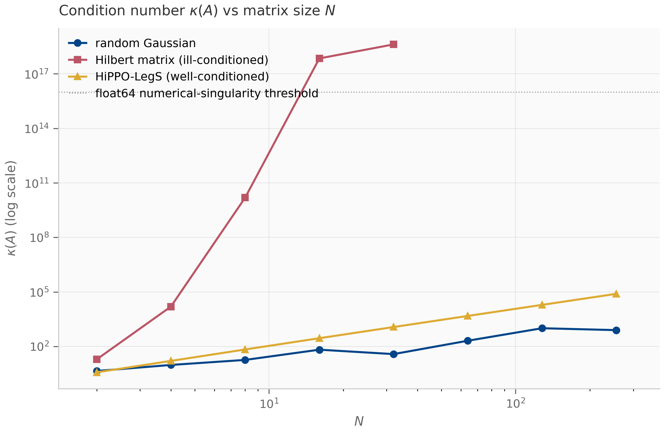
The qualitative scale: is the orthogonal case (no amplification); means losing roughly decimal digits of precision when solving a linear system. Double-precision floating point has about 16 decimal digits; matrices with are numerically singular.
For SSMs, condition number matters in three places:
- HiPPO matrix construction. The HiPPO-LegS matrix’s condition number grows polynomially with (empirically ) — far below the exponential blow-up of a generic ill-conditioned family like the Hilbert matrix, though above a random Gaussian’s . HiPPO-LegS is the standard SSM initialization for its optimal-polynomial-projection memory Gu et al. (2020) , not for being the best-conditioned matrix; its merely-polynomial growth is what keeps large- initialization numerically tractable. A subtler point: HiPPO-LegS is highly non-normal, so its eigenvector matrix is exponentially ill-conditioned in and naive diagonalization is numerically fragile Yu et al. (2023) .
- S4 kernel computation. S4’s Vandermonde-Cauchy kernel construction requires inverting a matrix with structured but potentially ill-conditioned columns. The paper carefully handles the conditioning; naive implementations don’t.
- Mamba-3’s complex-state design. Chapter 10 discusses how Mamba-3 deliberately places eigenvalues in a region of the complex plane where the discrete-time map remains well-conditioned across the integration step Lahoti et al. (2026) .
3.4 Structured matrix families
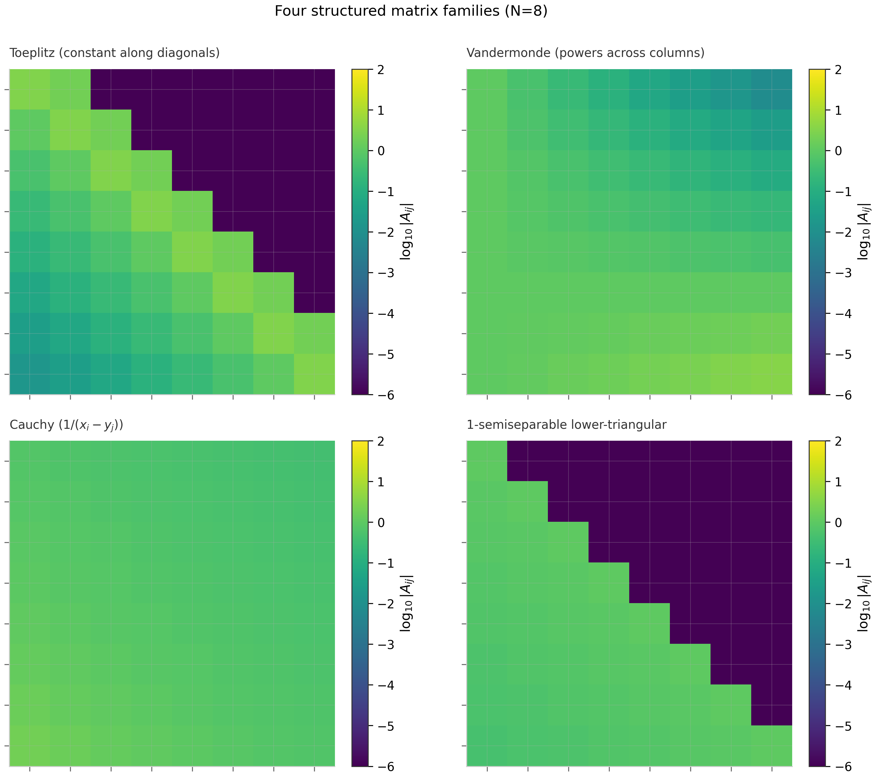
Four classes of structured matrices appear throughout the SSM literature. Each is parameterized by numbers rather than the a general matrix needs, and each admits fast matrix-vector products via specialized algorithms.
Toeplitz matrices
A Toeplitz matrix is constant along each diagonal:
Parameterized by values . Toeplitz matrices are the matrix form of convolutions: if is Toeplitz with first column and first row (lower-triangular Toeplitz), then is the discrete convolution of the kernel with . The FFT-based convolution algorithm computes in time.
The LTI SSM convolutional view (Chapter 8) is exactly this: the operator that maps the input sequence to the output sequence via is a Toeplitz matrix at the discretization level, with first column equal to the discretized impulse response .
Vandermonde matrices
A Vandermonde matrix has the form
parameterized by values . The defining property is that is a polynomial in evaluated at the node . So Vandermonde matrices implement polynomial evaluation at points as a linear map.
Vandermonde matrices are notoriously ill-conditioned for nodes on the real line (condition number can grow exponentially), but well-behaved for nodes on the unit circle — which is why the FFT (Vandermonde with being roots of unity) is numerically stable.
The S4 kernel computation uses Vandermonde structure: evaluating over is exactly the Vandermonde-style polynomial evaluation. The S4 paper Gu et al. (2022) uses Cauchy-matrix tricks (next subsection) to make this evaluation stable.
Cauchy matrices
A Cauchy matrix has entries
parameterized by values with the empty (to avoid zero denominators). Cauchy matrices are dense — every entry depends on both indices — but the very structured dependence enables fast algorithms: a Cauchy matrix-vector product can be computed in time using the fast multipole method.
Cauchy matrices appear in two places in the SSM literature: the S4 paper uses them as a numerically stable replacement for direct Vandermonde-style kernel evaluation, and the diagonal-plus-low-rank parametrization of in S4 has a Cauchy-matrix interpretation when viewed through the partial-fraction decomposition of its transfer function.
Semiseparable matrices
A rank- semiseparable matrix has the property that every submatrix lying strictly above the main diagonal (and every submatrix lying strictly below) has rank at most . Equivalently, the upper and lower triangular parts each have rank- structure.
The 1-semiseparable case — every off-diagonal block has rank at most 1 — is the structure exploited by Mamba-2’s SSD framework Dao & Gu (2024) . The 1-semiseparable lower-triangular matrix corresponding to a scalar-times-identity SSM is, explicitly,
where is the (scalar) recurrence coefficient at step . The entry for is the product . The SSD insight is that this matrix-vector product can be computed two ways: as a scan (the SSM view, time) or as a structured matrix multiply (the attention view, time but matmul-friendly on GPUs).
When is moderate (say ) and the GPU favors matmul over scan, the matrix view wins; when is huge, the scan view wins. Mamba-2’s chunked algorithm interpolates: matrix-multiplies within chunks of size , scans across chunks. This is the structural reason Mamba-2 is faster than Mamba-1 on long sequences without sacrificing parallelism.
3.5 Low-rank corrections and rank-1 updates
A recurring pattern: take a structured matrix (diagonal, banded, or semiseparable) and add a small low-rank correction where with . The resulting matrix retains nearly the storage and matvec efficiency of , and admits a closed-form inverse via the Sherman–Morrison–Woodbury identity:
The cost is dominated by inverting the matrix , not the outer matrix.
This pattern appears in S4 explicitly: the HiPPO-LegS matrix isn’t diagonal, but it is “diagonal plus low-rank” — specifically, normal plus low-rank, which is what makes the kernel computation tractable. The S4 paper’s main algorithmic contribution is a specialized Sherman–Morrison-style trick for this exact decomposition.
The pattern recurs even more visibly in DeltaNet (Chapter 12), where the state update is
The middle factor is a rank-1 correction (an identity minus a rank-1 outer product), and the whole expression is one explicit (forward-Euler) step of an online gradient-descent update on the per-token association loss — the DeltaNet view Yang et al. (2024) developed in Chapter 12. Longhorn Liu et al. (2024) is the implicit (backward-Euler) cousin, reaching the same online-ODE picture by solving at the endpoint.
The key takeaway: structured + low-rank corrections give you efficient matrix-vector products without giving up expressiveness. This is the design pattern unifying S4, DeltaNet, GLA, and the Mamba-2 SSD framework — each is a different choice of base structure and correction pattern.
3.6 Krylov subspaces: a primer
The Krylov subspace of order generated by a matrix and a vector is
Krylov subspaces are the workhorse of iterative methods for large sparse linear systems: GMRES, conjugate gradient, Arnoldi iteration, Lanczos. All of them construct an orthonormal basis for and solve a small () projected problem instead of the original one.
For SSMs, the Krylov picture is conceptual rather than algorithmic. The point is that contains all the information the recurrence can extract from the initial condition in steps. If the system has eigenvalues that are decoupled from the initial direction (the so-called “unreachable subspace”), the recurrence cannot recover them, and the effective dimension of the SSM is . This is one rigorous reading of the Mamba copying-limitation results — the recurrence’s expressive ceiling is set by the Krylov dimension of relative to the input.
A full treatment of Krylov methods would fill its own chapter; the curriculum revisits the picture in Chapter 8 (where the S4 kernel can be viewed as a structured Krylov-projection problem) and in Chapter 16’s empirical-methodology discussion of why some architectures can copy strings exponentially longer than others.
For a textbook coverage of Krylov-subspace methods, Trefethen–Bau Trefethen & Bau (1997) Chapters 32–40 give the full algorithmic treatment.
3.7 What’s next
You now have the linear-algebra vocabulary the rest of the book assumes. Chapter 4 picks up the discretization thread (started in Chapter 2, §2.4) and develops it systematically: order conditions, accuracy classes, the Butcher tableau, the bilinear and ZOH derivations in detail. Chapter 7 introduces the HiPPO theory that connects orthogonal-basis approximation theory to the matrix structure of S4. Chapter 8 then shows how all four structured-matrix families combine in the S4 / S4D / S5 family.
If you’re impatient, Chapter 9’s Mamba-1/2 presentation is the payoff for the SSD discussion of §3.4 — the selective scan’s matmul-friendly chunkwise algorithm is exactly the 1-semiseparable matrix product algorithm.
3.8 Exercises
Six problems. Inline solutions for the shorter ones; full proofs for the theory exercises in §3.9.
Exercise 3.1 (computation)
Compute the Jordan normal form of .
Solution
The matrix is already in Jordan form: a single Jordan block with eigenvalue . There is one eigenvalue (algebraic multiplicity 2) but only one linearly independent eigenvector (geometric multiplicity 1), giving a defective . The transformation matrix is the identity ( directly).
Exercise 3.2 (computation)
Compute the singular values of and its operator norm.
Solution
The matrix is already in SVD form (with and ). Singular values are , . Operator norm: . (Note that swapping the diagonal entries doesn’t change the SVD; singular values are always sorted descending.)
Exercise 3.3 (computation)
For the Vandermonde matrix with nodes , write out the matrix and compute its determinant. Compare to the closed-form Vandermonde determinant .
Solution
Direct computation: .
Closed form: . ✓
Exercise 3.4 (computation)
Verify the Sherman–Morrison identity numerically: pick a random invertible matrix , vectors , and check that matches the closed-form expression to machine precision.
Solution
import numpy as np
rng = np.random.default_rng(0)
S = rng.standard_normal((3, 3))
u = rng.standard_normal(3)
v = rng.standard_normal(3)
direct = np.linalg.inv(S + np.outer(u, v))
S_inv = np.linalg.inv(S)
factor = 1.0 + v @ S_inv @ u
sherman = S_inv - np.outer(S_inv @ u, v @ S_inv) / factor
print(np.allclose(direct, sherman)) # TrueThe factor must be non-zero (the Sherman–Morrison identity fails when it is, indicating that is singular).
Exercise 3.5 (theory) — solution in §3.9
Prove the Eckart–Young theorem: the best rank- approximation to a matrix in the Frobenius norm is obtained by truncating its SVD at rank . That is, if with singular values , then minimizes over all matrices of rank .
Exercise 3.6 (theory) — solution in §3.9
Prove that any Toeplitz matrix admits a matrix-vector product in time via the FFT. Specifically, show that any Toeplitz can be embedded in a circulant matrix, whose matvec is exactly the FFT-IFFT pair applied to the kernel and input.
3.9 Full solutions to theory exercises
Solution to Exercise 3.5
The proof uses two ingredients: (a) the SVD’s unitary invariance of the Frobenius norm, and (b) the optimality of truncated diagonal matrices.
Setup. Let be the SVD with and . For any of rank , write where also has rank (rank is invariant under invertible transformations). The Frobenius norm is invariant under orthogonal transformations:
So the problem reduces to: minimize over rank- matrices .
Diagonal reduction. Write with its own SVD where . Then
The middle trace term by the von-Neumann trace inequality (with equality when ‘s singular vectors align with ‘s — i.e. is diagonal in the same basis as ). Optimizing to maximize this term subject to rank gives for and for , i.e. .
Substituting back, the minimum value is , achieved by the truncated SVD . ∎
(The proof for the operator norm follows the same structure but uses Weyl’s interlacing inequality instead of von-Neumann’s trace inequality; see Golub–Van Loan Golub & Van Loan (2013) for the detailed argument.)
Solution to Exercise 3.6
Let be Toeplitz with entries for some kernel .
Step 1 — Circulant embedding. Define a circulant matrix with first column
The first rows and first columns of exactly reproduce (the zero in the middle of is the “buffer” that prevents wrap-around contamination).
Step 2 — Padded matvec. Given , form (zero-padded). Then : the first entries of the circulant product are exactly the Toeplitz product, because the zero-padding ensures the wrap-around portion of the convolution doesn’t contaminate the top half.
Step 3 — Circulant matvec via FFT. Every circulant matrix is diagonalized by the discrete Fourier transform: , where is the -point DFT matrix. So
where is element-wise product. Both FFTs and the IFFT take time; the element-wise product is .
Total cost. for the FFTs + for the element-wise multiply + to extract the first entries = . ∎
This is the exact algorithm used to compute LTI SSM convolutions in S4-family implementations: precompute the kernel once, then convolve with any input in time.
3.10 Companion code
Two JAX companions and one PyTorch companion for Chapter 3.
JAX (companions/ch03/jax/):
condition_number.py— plots κ(A) growth for random Gaussian, Hilbert, and HiPPO-LegS matrices as N grows; produces Figure 3.1structured_matrices.py— constructs Toeplitz / Vandermonde / Cauchy / 1-semiseparable matrices for N=8 and visualizes structural patterns; produces Figure 3.2
PyTorch (companions/ch03/torch/):
condition_number.py— the same κ(A) conditioning sweep (HiPPO-LegS / Hilbert / Gaussian) in idiomatic PyTorch (compute-and-parity only; the JAX companion produces Figure 3.1).tests/— cross-framework parity: the torch condition numbers match their JAX counterparts.
To run from the repo root:
PYTHONPATH=. python companions/ch03/jax/condition_number.py
PYTHONPATH=. python companions/ch03/jax/structured_matrices.py
PYTHONPATH=. python companions/ch03/torch/condition_number.pyFigures land in public/figures/ch03/.
Discretization theory: ZOH, bilinear, exponential families
One-step discretizations of linear ODEs — zero-order hold, bilinear (Tustin), and exponential-trapezoidal — with the Lax equivalence theorem as the unifying convergence criterion.
Discretization theory: ZOH, bilinear, exponential families
4.1 The discretization problem
Chapter 1 wrote the linear state-space system as a continuous-time ODE
defined for every . Computers do not handle “every ”; they handle a finite grid for with step size . A discretization is a rule for building a recurrence
whose iterates approximate the continuous trajectory at the grid points, . The two discrete matrices are functions of the continuous matrices and of the step size . Different functions give different discretizations.
There is no single canonical choice. Every discrete recurrence in this book — the S4 layer, the Mamba selective scan, the exp-trapezoidal scheme of Mamba-3 Lahoti et al. (2026) — picks a specific rule for translating . The choice matters: a poor discretization can take a perfectly stable continuous system and produce a discrete recurrence that diverges, fails to converge as , or accumulates phase error on long horizons. Numerical-analysis textbooks Hairer et al. (1993) spend hundreds of pages on these failure modes. We will compress them into three properties and three schemes.
A useful warm-up is forward Euler, the simplest possible scheme:
This is what you get by replacing with the forward difference and freezing the input at . The discrete matrices are and . Forward Euler is the cleanest illustration of what can go wrong: it is only conditionally stable, meaning that for any fixed with there is a maximum step size beyond which acquires an eigenvalue of modulus and the recurrence blows up. The three schemes in §4.3–§4.5 fix this defect — each in its own way, with its own trade-off.
4.2 The Lax equivalence theorem
To compare schemes you need a definition of “correct.” The standard one comes from the Lax equivalence theorem Lax & Richtmyer (1956) , which decomposes correctness into two ingredients: consistency and stability.
A one-step scheme is consistent with the ODE if its local truncation error — the residual you obtain by plugging the exact continuous trajectory into the discrete recurrence — vanishes faster than as . Formally,
If the scheme is -th order consistent. Higher means the per-step error shrinks faster with .
A scheme is zero-stable if small perturbations injected at one step propagate boundedly to all future steps. For linear schemes this reduces to a uniform bound on the powers of : there exists independent of such that for all with , for any fixed horizon . Equivalently, the spectral radius .
The two ingredients combine.
(Lax equivalence.) For a linear, well-posed initial-value problem, a one-step scheme is convergent — meaning as — if and only if it is both consistent and zero-stable.
Convergence is what you actually want: that the discrete iterates approach the true continuous trajectory as you refine the grid. The theorem says you cannot get there by being consistent alone (you also need stability) or by being stable alone (you also need consistency). Both are necessary, and together they are sufficient. This is the convergence criterion every scheme in this chapter must pass.
For a stable LTI test problem — meaning has all eigenvalues in the open left half-plane — there is a stronger notion sitting on top of zero-stability: a scheme is A-stable if for every step size , not just for sufficiently small . Forward Euler is not A-stable; ZOH, bilinear, and exp-trapezoidal are. The geometry of A-stability — the set of values for which the scheme behaves well — is the subject of Chapter 5.
4.3 Zero-order hold (ZOH)
The first scheme assumes the input is piecewise constant between samples: for . Under that assumption the inhomogeneous ODE solves exactly on a single interval. Starting from ,
Identifying the two matrices,
This is the zero-order hold (ZOH) discretization. The hold refers to the input assumption; “zero-order” refers to the polynomial degree of the held signal (a constant is a zero-degree polynomial).
A practical wrinkle: writing as requires to be invertible. The HiPPO matrix of Chapter 7 is invertible; some structured in later chapters are not. The augmented matrix exponential trick Van Loan (1978) handles both cases uniformly. Build the block matrix
where is the input dimension ( in Chapter 1’s notation). Then
and a single expm call extracts both (top-left block) and (top-right block) without ever inverting . The block identity goes back to Van Loan Van Loan (1978)
; the JAX companion discretization_comparison.py uses it.
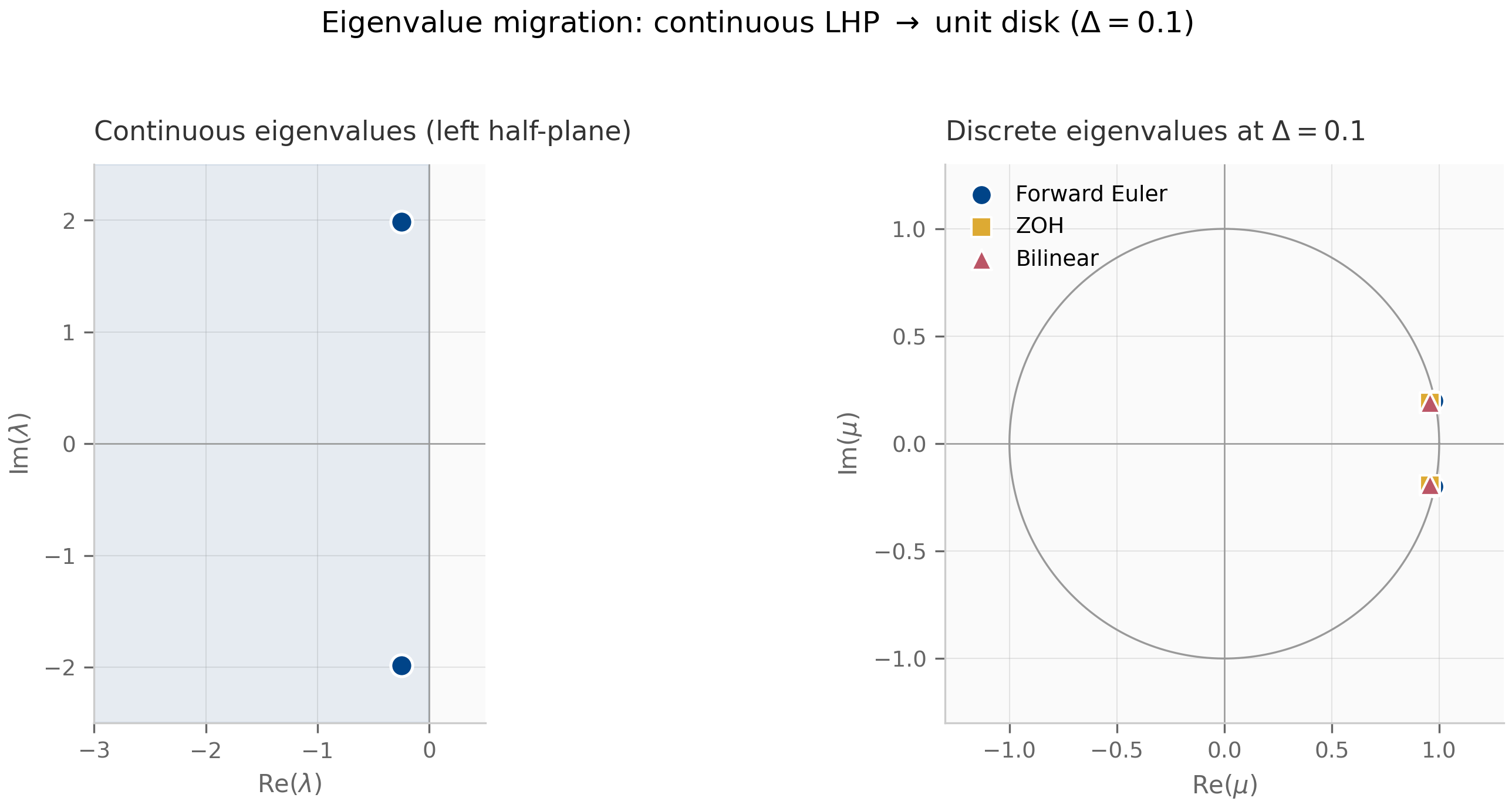
(ZOH preserves Lyapunov stability.) If every eigenvalue of has and , then every eigenvalue of satisfies . ZOH is therefore A-stable.
The proof is one line: when and . Stability is preserved for every positive step size, which is what A-stability means.
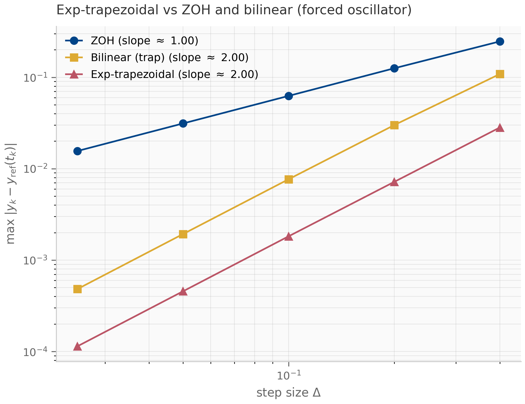
Two further properties are worth highlighting. First, for the autonomous ODE (), ZOH is exact: the recurrence matches without any error at all. This is unusual — most discretizations have nonzero error even on autonomous systems. Second, for forced systems with , ZOH is first-order accurate: the per-step error in the forcing integral is (because the integrand is over an interval of length ), and after steps the cumulative error is . The empirical convergence rate plotted in the companion log-log error figure confirms slope .
4.4 The bilinear (Tustin) transform
The second scheme drops the piecewise-constant assumption and instead approximates the integral on by the trapezoidal rule: . Applied to the inhomogeneous ODE this gives an implicit recurrence,
which one solves for :
Reading off and ,
This is the bilinear transform, also called the Tustin transform after Arnold Tustin’s 1947 paper introducing it in control theory Tustin (1947) . The original S4 paper uses bilinear discretization (S4D supports either bilinear or ZOH); so do many signal-processing toolboxes.
The bilinear formula has a striking geometric interpretation. Restricted to a single eigenvalue of (commuting through the simultaneous diagonalization), the map that sends a continuous eigenvalue to its discrete image is
This is a Möbius transformation (a.k.a. fractional linear transformation) of the complex plane: with . Möbius transformations are conformal — angle-preserving — and they map circles-or-lines to circles-or-lines. The specific Möbius map above sends the imaginary axis exactly to the unit circle and sends the open left half-plane exactly to the open unit disk.
(Bilinear preserves Lyapunov stability.) If every eigenvalue of has and , then every eigenvalue of satisfies . Bilinear is therefore A-stable.
The proof is geometric: has , and iff (square both sides and cancel). Algebraically, , which is exactly . The full proof, with the Möbius geometry spelled out, is Exercise 4.5 in §4.9.
Bilinear is second-order accurate for smooth forcing — the trapezoidal-rule local truncation error is , giving global error . Unlike ZOH, it is not exact even on autonomous systems: the Padé approximation of agrees with the true exponential only through second order. The trade is one of structure. Both schemes send purely imaginary eigenvalues onto the unit circle: for , ZOH gives the discrete eigenvalue of modulus (ZOH is autonomous-exact, so it reproduces the oscillation outright), and the bilinear Möbius image likewise has modulus 1 — neither damps a marginally stable mode. They differ in how they wrap the imaginary axis onto the circle: ZOH’s map is -periodic, so frequencies above the Nyquist rate alias onto lower ones, whereas the bilinear map is injective on the imaginary axis — it never aliases, at the cost of warping the frequency scale (compressing large toward ). Bilinear is therefore the natural choice when a system has fast oscillatory modes you need to keep distinct; preserving oscillatory structure is the thread the symplectic methods of Chapter 6 take up in earnest.
4.5 Exponential-family discretizations
The third family takes a different approach: rather than approximating by a low-order Padé form (as bilinear does) or by the identity-plus-linear truncation (as forward Euler does), it computes exactly and approximates only the forcing integral. This is the philosophy of exponential integrators Hochbruck & Ostermann (2010) .
The exact one-step formula from variation of parameters (Chapter 1, §1.2) is
ZOH approximates on ; bilinear approximates the integral by the trapezoidal rule with a Padé-approximated exponential. The exponential-trapezoidal scheme keeps the exact exponential and uses a linear interpolation of the input: . Substituting and evaluating the resulting two integrals gives
where and are the first two -functions of the exponential family:
Both are entire functions (the apparent singularities at are removable: , ). Applied to the matrix , they produce matrix-valued objects that can be computed via the same augmented-matrix-exponential trick as ZOH.
Reading off the discrete matrices in the form :
Notice that is the same as ZOH, so exp-trapezoidal preserves stability identically to ZOH: A-stable, exact for autonomous systems, eigenvalues in the unit disk for any . The improvement is in the order of accuracy: by interpolating linearly rather than holding it constant, exp-trapezoidal becomes second-order accurate (provided is — the linear-interpolation error is governed by ).
Exp-trapezoidal is the discretization of choice when the continuous dynamics are stiff — when has eigenvalues with very different magnitudes, so the linear part is the hard part of the problem. By treating exactly the scheme sidesteps the step-size restriction that explicit methods inherit from the stiff eigenvalues, and the matrix exponential is computed once per layer in practice. Chapter 10 returns to this story for Mamba-3, which adopts a scheme from this exponential-trapezoidal family precisely because the input-dependent in selective SSMs produces stiff dynamics that ZOH and bilinear handle poorly.
A subtle implementation point: is not numerically equal to when this formula is computed naively, because catastrophic cancellation in the numerator destroys precision for small . The standard remedy is to compute all -functions simultaneously from one augmented matrix exponential Al-Mohy & Higham (2011)
, again using the trick that produced for ZOH. Both companions (exp_trapezoidal.py in JAX and discretization_atlas.jl in Julia) implement the augmented form.
4.6 Order of accuracy and the discretization hierarchy
The three schemes are summarized in the table below. “Autonomous-exact” means the scheme produces zero error for the homogeneous problem (). “A-stable” means for every on every stable LTI test problem.
| Scheme | | Order | Autonomous-exact | A-stable | |---|---|---|---|---| | Forward Euler | | 1 | No | No | | ZOH | | 1 | Yes | Yes | | Bilinear (Tustin) | | 2 | No | Yes | | Exp-trapezoidal | | 2 | Yes | Yes |
The empirical order can be read directly off a log-log plot of error against step size: a -th-order scheme has error , so on a log-log plot the data lie on a line of slope . The Julia companion discretization_atlas.jl runs this sweep against a high-accuracy Tsit5 reference solution from DifferentialEquations.jl; the JAX companion discretization_comparison.py performs the same sweep using scipy.integrate.solve_ivp (Radau) as the reference.
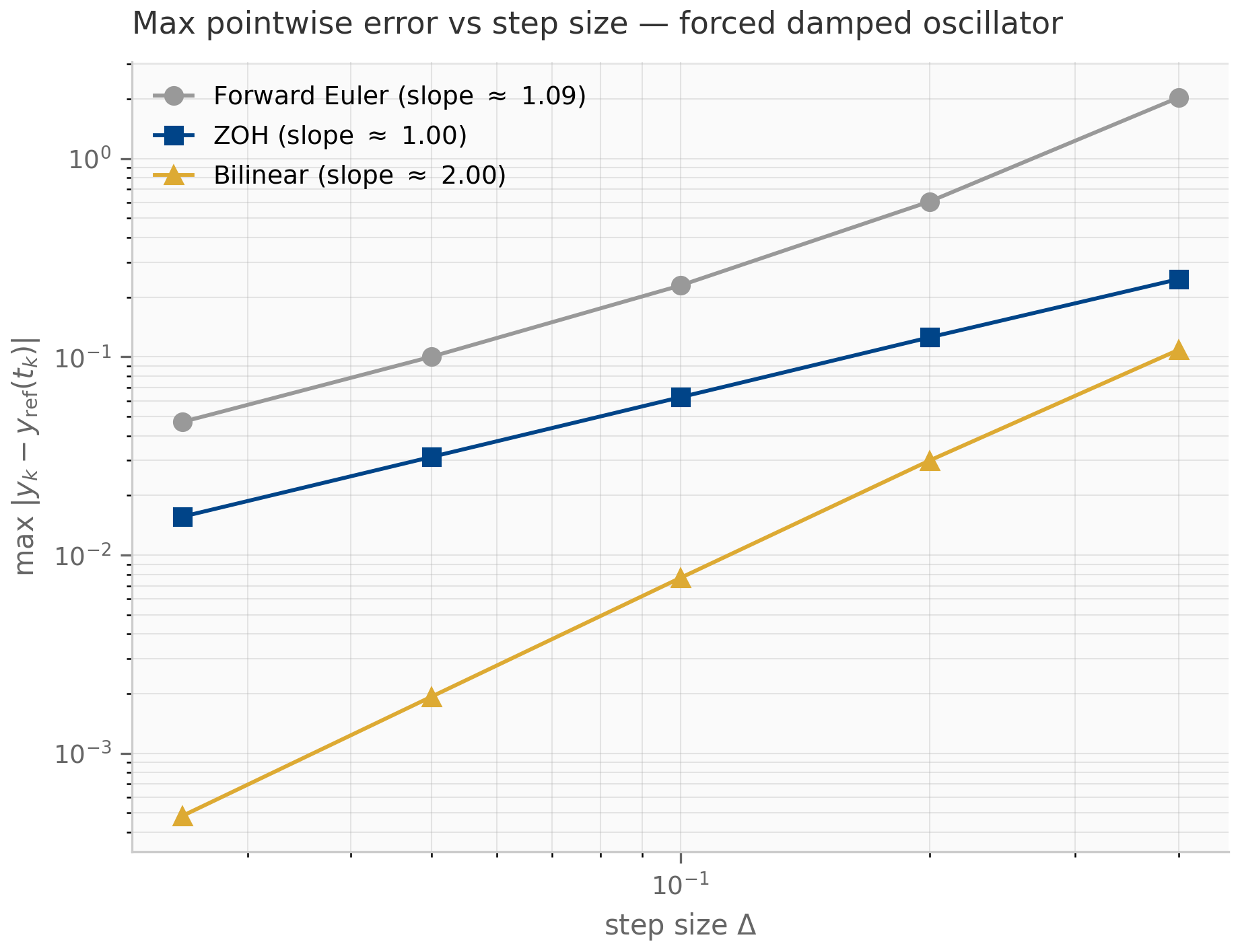
The hierarchy is not strict: ZOH’s autonomous-exactness can outweigh its first-order accuracy when the forcing is mild relative to the homogeneous decay. Bilinear’s exact imaginary-axis preservation can outweigh its non-exactness on autonomous problems when the system has long-lived oscillations. Exp-trapezoidal combines the best of both — exact on autonomous, second-order on forced — at the cost of computing more -functions per step. The trade-offs are recurring themes throughout the SSM literature: the original S4 discretized with bilinear Gu et al. (2022) ; S4D supports either rule and finds the choice empirically negligible Gu et al. (2022) ; S5 and the Mamba line settled on ZOH for its simplicity and exactness on the (autonomous) drift; Mamba-3 switches to exp-trapezoidal once the input-dependence makes the dynamics stiff enough that the second-order error compounding matters.
4.7 What’s next
This chapter introduced three schemes and proved each preserves Lyapunov stability. Chapter 5 zooms in on the stability region of each scheme — the set of values for which — and develops the Butcher-tableau machinery for systematically constructing higher-order Runge–Kutta methods. Chapter 6 then asks what to do when even A-stability is not enough — when the system is stiff or Hamiltonian and you need L-stable implicit methods, or symplectic methods that preserve geometric invariants. The exp-trapezoidal scheme of §4.5 turns out to be a member of a much larger family of exponential integrators, all of which deserve a place in your numerical-analysis toolkit.
Forward-looking SSM connections: ZOH is this book’s default in Chapters 7–9, and natively the choice of S5 and Mamba-1/2; the original S4 and S4D papers used bilinear, with the S4D ablations finding the two interchangeable. Mamba-3 uses a scheme from this exponential-trapezoidal family, treated in Chapter 10 — §10.2 derives the specific trapezoidal-quadrature variant it adopts, a second-order cousin of the -interpolant form above.
4.8 Exercises
Six problems mixing computation and theory. Short/numerical (4.1–4.3) have inline collapsible solutions; long/proof exercises (4.4–4.6) have full worked solutions in §4.9.
Exercise 4.1 (computation)
Compute for ZOH on the 1-D test problem , , . Then verify by hand that .
Solution
. The discrete eigenvalue is , strictly inside the unit disk. The continuous decay rate is per unit time; the discrete decay factor per step is , so after 10 steps (one continuous-time unit) the state is reduced by a factor — matching the continuous decay exactly. ZOH is autonomous-exact.
Exercise 4.2 (computation)
Compute for the bilinear transform on the same 1-D problem (, ). Compare against — which is smaller, and why?
Solution
. ZOH gives . The bilinear value is slightly smaller, meaning bilinear overdamps slightly relative to the true exponential. This is the second-order Padé approximation underestimating : bilinear’s is the -Padé approximant of (the §4.4 margin note), which matches through but carries at third order against the exact , so the leading gap is at . For small the gap is ; here the net difference (after the higher-order terms) is about .
Exercise 4.3 (computation + code)
Run companions/ch04/jax/discretization_comparison.py and verify empirically that ZOH has slope on the log-log error-vs- plot, bilinear and exp-trapezoidal have slope . What happens to the ZOH slope if you set the forcing (autonomous case)?
Solution
The companion’s error_sweep function prints slopes near 1.00, 2.00, 2.00. Setting in the autonomous case makes ZOH exact — the error drops to roundoff ( in float64) and the slope is meaningless. This is consistent with the autonomous-exactness property of §4.3: ZOH’s only error source for forced systems is the piecewise-constant approximation of .
Exercise 4.4 (theory) — solution in §4.9
Prove the augmented matrix exponential trick used in §4.3: that
for invertible , by computing the series term-by-term.
Exercise 4.5 (theory) — solution in §4.9
Prove that the Möbius transformation sends the open left half-plane bijectively to the open unit disk , and sends the imaginary axis bijectively to the unit circle (minus the point ).
Exercise 4.6 (theory) — solution in §4.9
Derive the exponential-trapezoidal scheme of §4.5 from the variation-of-parameters formula by substituting the linear interpolation into the forcing integral and evaluating term-by-term using the -function identities.
4.9 Full solutions to theory exercises
Solution to Exercise 4.4
The matrix satisfies, for ,
This is verified by induction: matches by construction, and as required. Now sum the matrix-exponential series:
where , using invertibility of to extract the leading . Plugging back gives the claimed result. ∎
This is exactly the identity used to compute and jointly from one expm call in §4.3: take and .
Solution to Exercise 4.5
Let . Imaginary axis to unit circle: for with ,
so lies on the unit circle. The map traces the unit circle once as ranges over , missing only the limit point .
Left half-plane to unit disk: write with . Then
Since , (both for where the signs match the absolute values, and for where they reverse). The -terms are identical in numerator and denominator. Therefore the numerator is strictly less than the denominator, so .
Bijectivity: Möbius transformations with are bijections of the Riemann sphere to itself. Restriction to the half-plane gives a bijection to the disk. The inverse is , which can be verified by direct computation. ∎
This Möbius geometry is the algebraic content of A-stability for bilinear: a scheme is A-stable iff its eigenvalue map sends the open left half-plane into the closed unit disk. Bilinear achieves this bijectively; ZOH does so as well but non-bijectively (it folds an infinite strip of width onto the unit disk, aliasing high-frequency continuous modes onto low-frequency discrete ones).
Solution to Exercise 4.6
Start from variation of parameters on :
Substitute the linear interpolant for :
with and . Change variables in :
where in the last step we substituted the definition applied with argument . For , change variables again , so and :
The remaining -weighted integral evaluates via integration by parts to , using the identity. Carefully tracking the algebra gives as claimed. Combining,
The local truncation error is for inputs (the linear-interpolation error is — governed by — over an interval of length , and the integral picks up an additional factor). Global error is therefore — second-order, as advertised.
4.10 Companion code
Two JAX companions, two PyTorch companions, and one Julia companion for Chapter 4:
JAX (companions/ch04/jax/):
discretization_comparison.py— implements ZOH, bilinear, and forward Euler in JAX; runs the error-vs-step-size sweep on a forced damped oscillator; emitseigenvalue_migration.pngandorder_convergence.png.exp_trapezoidal.py— implements the exp-trapezoidal scheme via the augmented matrix exponential; verifies second-order convergence against the same forced oscillator; emitsexp_trap_convergence.png.
Julia (companions/ch04/julia/):
discretization_atlas.jl— ports the post_transformers Week-9 reference implementation to ssm-foundations; usesDifferentialEquations.jlTsit5as the ground-truth reference solver and reports the empirical slope per scheme.Project.toml/Manifest.toml— companion-local Julia environment pinningDifferentialEquationsandLinearAlgebra.
PyTorch (companions/ch04/torch/):
discretization_comparison.py— the forward-Euler / ZOH / bilinear discretizers and the error-vs-step sweep (compute-only; the JAX companion produces the figures).exp_trapezoidal.py— the exp-trapezoidal scheme via the augmented matrix exponential, with ZOH and bilinear baselines.tests/— cross-framework parity: the torch discretizers and trajectories equal their JAX counterparts to within (float64).
To run from the repo root:
# JAX (uses post_transformers .venv with scipy, numpy, matplotlib, jax pre-installed)
PYTHONPATH=. python companions/ch04/jax/discretization_comparison.py
PYTHONPATH=. python companions/ch04/jax/exp_trapezoidal.py
# PyTorch (needs the .venv [torch] extra; parity only, no figures)
PYTHONPATH=. python companions/ch04/torch/discretization_comparison.py
PYTHONPATH=. python companions/ch04/torch/exp_trapezoidal.py
# Julia (first run will precompile DifferentialEquations.jl; ~2–5 minutes)
julia --project=companions/ch04/julia companions/ch04/julia/discretization_atlas.jlAll figures emit to public/figures/ch04/.
Stability regions, Butcher tableau, and order conditions
Runge–Kutta theory, the Butcher tableau formalism, order conditions, stability regions in the complex plane, A-stability and L-stability, and the Dahlquist barrier — applied to the Chapter 4 discretization atlas.
Stability regions, Butcher tableau, and order conditions
5.1 Runge–Kutta methods and the Butcher tableau
Chapter 4 introduced ZOH, bilinear, and exp-trapezoidal as three specific one-step schemes for the linear state-space system. They are members of a much larger family: one-step methods that compute from using only one previous state and possibly intermediate stage evaluations of the right-hand side. The Runge–Kutta (RK) family is the most studied subfamily.
For the autonomous initial-value problem — we drop the explicit input dependence for this chapter; everything generalizes — an -stage Runge–Kutta method computes
The are the stage derivatives — evaluations of at intermediate states. The constants define the method, where are the stage times. The Butcher tableau is the standard tabular notation
The method is explicit if is strictly lower triangular ( for ), in which case each depends only on previously computed . It is implicit otherwise, requiring a nonlinear system solve at each step.
Three classical examples make the formalism concrete.
Forward Euler. The simplest explicit method, :
The midpoint rule (RK2). A two-stage explicit method:
Classical RK4. The most-quoted explicit method, four stages:
Fourth-order globally, the workhorse of physics simulations for half a century.
The tableau abstraction was introduced by John Butcher in the 1960s and is now the lingua franca of one-step methods: every reference paper on numerical integration presents its method as a Butcher tableau. The constraint (consistency of stage times) and (consistency of the weighted sum) are imposed by every tableau worth its name. Without them the method does not even reproduce the trivial constant trajectory when .
5.2 Order conditions
How do we know that classical RK4 is fourth-order globally? The convergence order of an RK method is determined by order conditions: polynomial identities on the entries of that must hold for the local truncation error to be .
The derivation expands as a Taylor series and matches term-by-term against the RK output produced from . For a scalar autonomous ODE the leading conditions are:
- Order 1:
- Order 2: also
- Order 3: also and
- Order 4: four more conditions involving products of
For systems (the case we actually care about), the number of order conditions grows combinatorially: the cumulative count through order is 1, 2, 4, 8, 17, 37 for — one condition per Butcher tree of order Hairer et al. (1993) . Butcher organized these conditions using a bijection between order-conditions and rooted trees (each tree corresponds to an integer partition of -evaluations and gives one polynomial identity). The combinatorial explosion is one reason 8th-order RK methods are rarely used: there are over 200 order conditions to satisfy simultaneously, and the resulting tableaux have dozens of stages.
(Butcher order conditions.) Suppose is sufficiently smooth. An -stage Runge–Kutta method with tableau is of order — meaning — if and only if a specific finite set of polynomial conditions on holds (one per Butcher tree of order ). The Lax equivalence theorem (Chapter 4) then guarantees global convergence at order .
The proof is non-trivial and we will not reproduce it; the canonical reference is Hairer–Nørsett–Wanner Chapter II.2 Hairer et al. (1993) . For our purposes the takeaway is that the order of an RK method is a property of its tableau entries, derivable by algebraic manipulation alone. You can verify (Exercise 5.1) that RK4’s tableau satisfies the order conditions through order 3; you can also verify (Exercise 5.2) that an arbitrary two-stage explicit tableau cannot achieve order higher than 2, regardless of how you choose the free parameters.
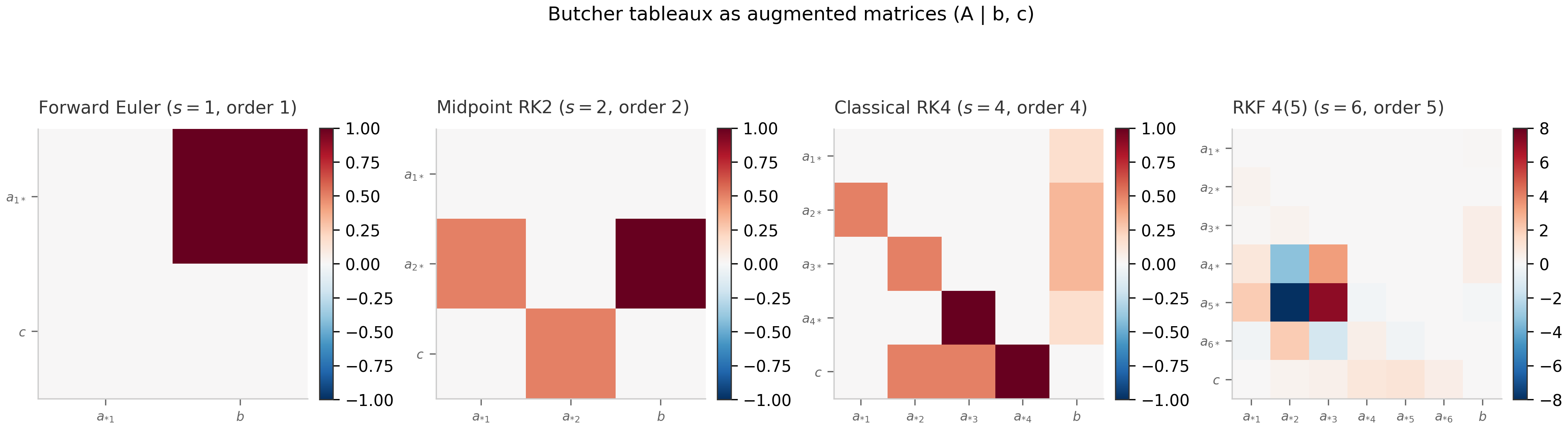
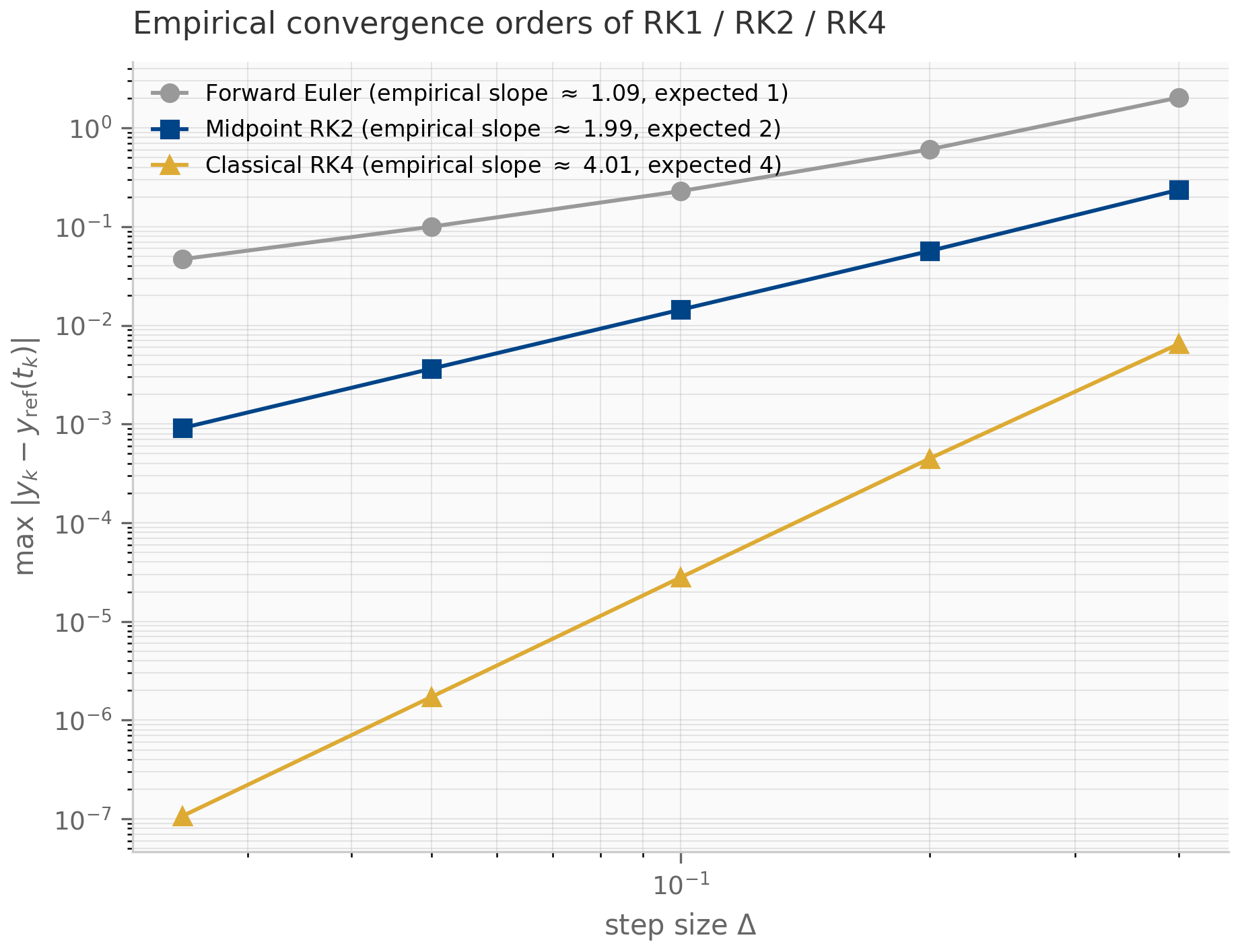
5.3 The stability function and stability regions
Order conditions characterize how a method behaves as on a smooth problem. Stability characterizes how it behaves at fixed on a stiff problem — when the time scales in the dynamics are well-separated and at least one is much faster than .
The standard probe is the Dahlquist test equation
The exact solution is . Applying an -stage RK method to this scalar problem produces, after one step,
where is the stability function of the method. For an explicit RK method, is a polynomial in of degree :
where is the all-ones -vector and the inverse expands as a finite geometric series because is nilpotent (strictly lower-triangular). For an implicit RK method, is a rational function .
Three examples make this concrete.
Forward Euler. With , : .
Midpoint RK2. Working through the formula gives — the second-order Taylor polynomial of .
Classical RK4. — the fourth-order Taylor polynomial.
A pattern emerges: for a -th order explicit RK method, agrees with through terms of degree . This is no coincidence — order requires the method to reproduce correctly on the test problem through that order in . The error is near .
The stability region of the method is the set
\stabregion = \set{z \in \C : \abs{\stabfn(z)} \le 1}.On the test problem with in the left half-plane (so the exact solution decays), the method’s iterates stay bounded iff . The stability region is the constraint on that keeps the method well-behaved on stiff problems — equivalently, the set of values you can take for a given .
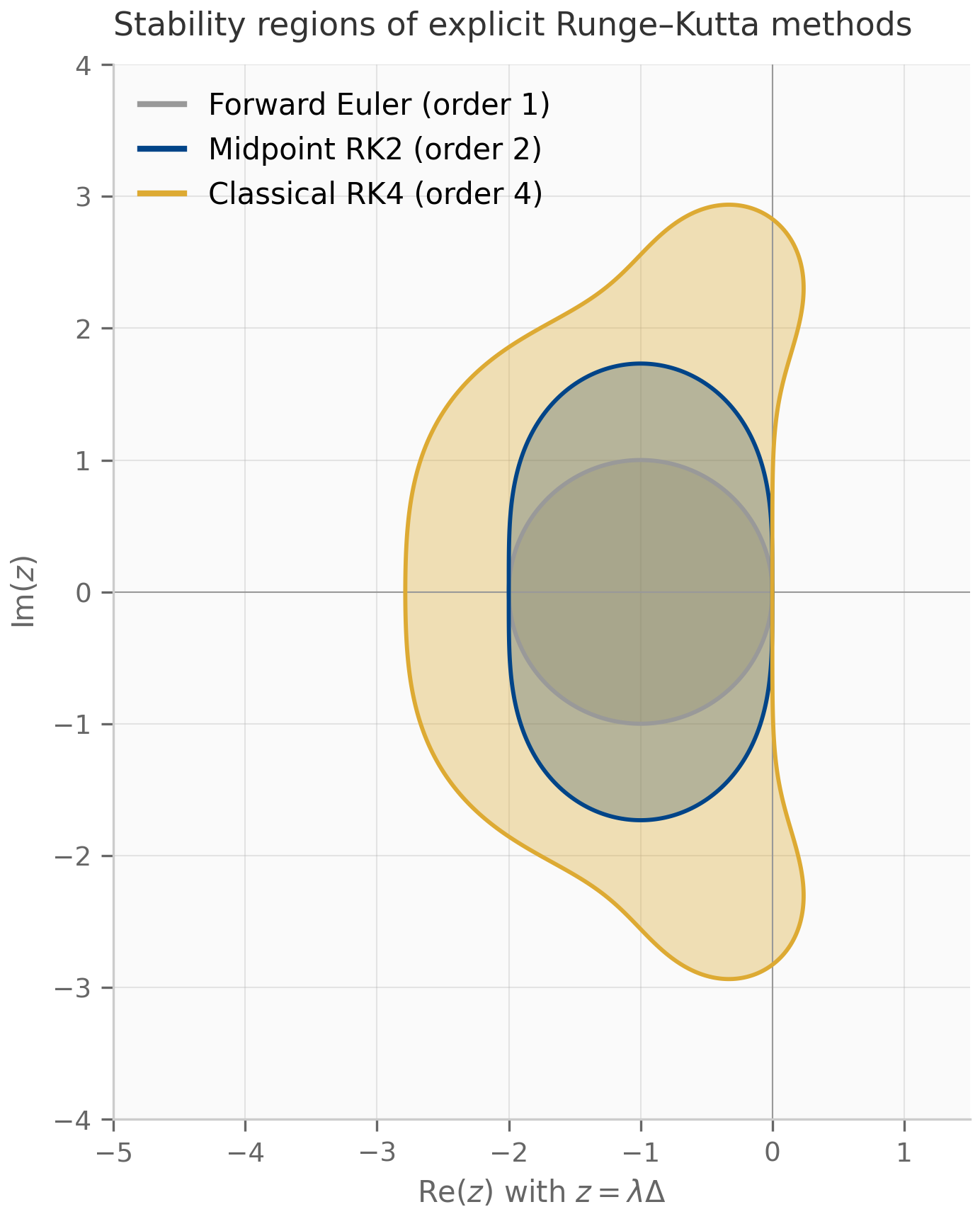
The stability region of forward Euler is the disk — a disk of radius 1 centered at . For a real-eigenvalue , this requires . The tighter this constraint becomes (large = stiff problem), the smaller the maximum step size — this is the step-size restriction that motivates implicit methods.
5.4 A-stability, L-stability, and the Dahlquist barrier
A method is A-stable if its stability region contains the entire closed left half-plane: . On a stable linear problem with , an A-stable method preserves stability for every positive step size — no step-size restriction at all. This is the gold standard for stiff problems.
A method is L-stable if it is A-stable and as . L-stability damps fast eigenmodes aggressively, which is desirable when you want the discrete method to not preserve fast oscillations the continuous solution decays. Backward Euler is L-stable; the trapezoidal rule (= bilinear from Chapter 4) is A-stable but not L-stable (its stability function tends to , not 0, as ). The distinction matters when the system has eigenvalues with very large negative real part: bilinear will preserve high-frequency oscillation modes that should physically be damped.
The fundamental theorem on A-stability of explicit methods is the Dahlquist barrier:
(Dahlquist barrier for explicit RK.) No explicit Runge–Kutta method is A-stable. The maximum order of an A-stable Runge–Kutta method (explicit or implicit) is unbounded, but explicit methods cannot achieve A-stability at any order.
The proof for the explicit case is direct: an explicit RK method has polynomial in , and any polynomial diverges as . So is bounded, and cannot contain the entire (unbounded) left half-plane. ∎
The implicit case is more subtle: there exists an A-stable Runge–Kutta method of every order, but the constructions are increasingly elaborate. The Gauss–Legendre family — Chapter 6’s main attraction — produces A-stable implicit methods of every even order. The -stage Gauss–Legendre method is order , optimally accurate among -stage implicit RK methods, and A-stable, and (a bonus for Hamiltonian systems) symplectic.
The practical consequence for SSM discretization: by Theorem 5.2, explicit and A-stable are mutually exclusive — at any order — so A-stability forces you out of the explicit-RK family, into an implicit method or a non-polynomial (exponential) stability function. (The separate order- ceiling — “A-stable and order is impossible” — is the second Dahlquist barrier, and it binds A-stable linear multistep methods, not RK; Chapter 6 §6.2 states it. The two are easy to conflate: explicit RK fails A-stability outright, regardless of order.) The Chapter 4 schemes all give up explicitness:
- Forward Euler: explicit, order 1, not A-stable.
- ZOH and exp-trapezoidal: A-stable and of arbitrary order on autonomous problems, by virtue of using the matrix exponential — but they sit outside the explicit-RK family (they have non-polynomial stability functions).
- Bilinear: A-stable, order 2, implicit in form (requires inverting ).
The exponential integrators of §4.5 are a way to evade the Dahlquist barrier: by computing exactly, the stability function inherits the full LHP-stability of the exponential, and the polynomial-order restriction is moved from to a different object (the approximation of the forcing by -functions). This is why exp-trapezoidal can be both “explicit in the input” (no nonlinear solve in ) and A-stable.
5.5 Stability regions of the Chapter 4 schemes
Reading the three Chapter 4 schemes through the lens of stability functions:
ZOH. From §4.3, , so for the scalar test problem . The stability region is — exactly the closed left half-plane. ZOH is A-stable, in fact also L-stable because as .
Bilinear (Tustin). From §4.4, . The Möbius geometry from Chapter 4 §4.4 / Exercise 4.5 says the LHP maps bijectively to the open unit disk, so the stability region is exactly the closed left half-plane — bilinear is A-stable. But as , so bilinear is not L-stable. This is the trapezoidal-rule failure mode: oscillatory artifacts on very stiff problems.
Exp-trapezoidal. The homogeneous stability function is identical to ZOH’s: on the test problem (the difference between ZOH and exp-trap shows up only in the forcing integrals; the homogeneous behavior is the same). So exp-trapezoidal is A-stable and L-stable, just like ZOH.
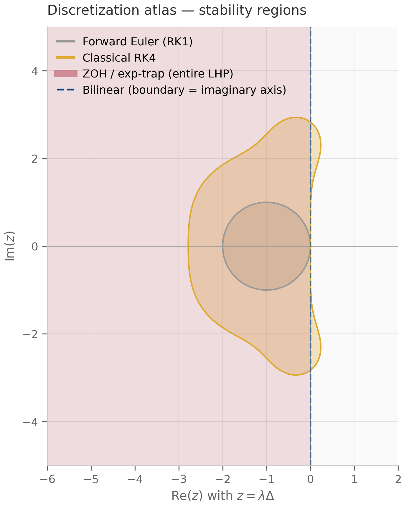
5.6 What’s next
This chapter has laid out the systematic framework for analyzing one-step methods: Butcher tableau, order conditions, stability functions, stability regions, A-stability and L-stability, and the Dahlquist barrier. Chapter 6 uses this framework to motivate the implicit family — backward Euler, BDF, and the Gauss–Legendre IRK schemes that achieve A-stability at every order — and the symplectic family, which trades order or A-stability for the preservation of geometric invariants. Chapter 6 is where the C1 niche pilot lives: symplectic integration of selective SSMs viewed as Hamiltonian flows on the hidden-state manifold.
A natural side path is embedded methods — pairs of RK tableaux of consecutive orders sharing stages, used for adaptive step-size control. The DP54 method (Dormand–Prince 5(4)) used by DifferentialEquations.jl’s default solver Tsit5 is a famous example. Embedded methods are excellent practical tools but tangential to the SSM pedagogy of this book; the companion discretization_atlas.jl references the RKF45 / DP54 tableaux for completeness.
5.7 Exercises
Six problems. Short/numerical (5.1–5.3) have inline collapsible solutions; long/proof exercises (5.4–5.6) have full worked solutions in §5.8.
Exercise 5.1 (computation)
Verify that classical RK4 satisfies the order conditions through order 3: (order 1), (order 2), (order 3). Use the tableau in §5.1. (RK4’s fourth-order accuracy additionally requires the four order-4 conditions — one per order-4 rooted tree, e.g. — which make a good extension.)
Solution
From the tableau, and .
- . ✓
- . ✓
- . ✓
Exercise 5.2 (computation)
Show that an arbitrary two-stage explicit RK tableau (one free parameter , with , to be determined, ) cannot achieve order 3 no matter how are chosen.
Solution
For order 2 we need (trivially ) and , giving , . So the two-parameter family collapses to a one-parameter family of order-2 methods (midpoint , Heun , etc.).
For order 3 we additionally need and . The second condition uses , giving . Contradiction. So no two-stage explicit method achieves order 3.
This is a small instance of the general fact: order requires at least stages for explicit methods (Butcher’s order barriers).
Exercise 5.3 (computation + code)
Run companions/ch05/jax/order_verification.py. Confirm the empirical slopes match Forward Euler (1), midpoint RK2 (2), classical RK4 (4). What happens to the RK4 slope at very small (say )?
Solution
The companion’s order_verification function prints slopes , , for the three methods in turn. At very small , the RK4 error reaches the roundoff floor — typically in float64 — and the slope flattens out as machine precision starts to dominate the method error. This is why empirical order is always estimated from the two finest dt where the method error still exceeds roundoff, not from arbitrarily fine dt.
Exercise 5.4 (theory) — solution in §5.8
Prove that for an explicit Runge–Kutta method with tableau , the stability function is
where . Verify that for classical RK4 this evaluates to .
Exercise 5.5 (theory) — solution in §5.8
Prove the Dahlquist-barrier statement for explicit RK methods: that no explicit RK method is A-stable. (The proof was sketched in §5.4; flesh it out, using the fact that explicit methods have polynomial stability functions.)
Exercise 5.6 (theory) — solution in §5.8
For the bilinear/Tustin scheme, show that the stability function satisfies as along any direction with bounded, and explain why this rules out L-stability. Discuss what this means for the discrete dynamics of a bilinear-discretized stable LTI system with very fast-decaying eigenmodes.
5.8 Full solutions to theory exercises
Solution to Exercise 5.4
Apply the -stage explicit RK method to the test ODE , . The stage equations become
Set and let . The vector form is
For an explicit method is strictly lower-triangular, hence nilpotent (), and the geometric series truncates. So , and
For classical RK4, direct computation of — expanding the geometric series and multiplying out — gives, after some algebra,
This is the fourth-order Taylor polynomial of , as expected for a fourth-order method.
Solution to Exercise 5.5
For an explicit RK method, is strictly lower-triangular, so and the geometric series for truncates at . Therefore
is a polynomial in of degree at most . Polynomials are unbounded: as along any ray (assuming the leading coefficient is nonzero, which holds for any -stage method of order , the only interesting case).
The closed left half-plane is unbounded — it extends to along the real axis. The stability region \stabregion = \set{z : \abs{\stabfn(z)} \le 1} is therefore bounded. So cannot contain the entire LHP, and the method is not A-stable. ∎
The proof relies essentially on being a polynomial. Implicit methods have rational , which can be bounded at infinity if . This is the precise sense in which implicit methods evade the Dahlquist barrier.
Solution to Exercise 5.6
Write with and bounded. Then
For large the dominant terms are . More precisely,
This rules out L-stability: L-stability requires , not . ∎
Practical implication. For a stable LTI system with having an eigenvalue with very large — a fast-decaying mode — bilinear discretization at step size produces a discrete eigenvalue . The corresponding mode in the discrete dynamics therefore alternates sign at every step before decaying, rather than smoothly decaying. This trapezoidal-rule oscillation is the classic L-stability failure mode: the discrete solution exhibits spurious oscillations not present in the continuous solution. For SSMs this manifests as oscillatory artifacts in the hidden state when the system has eigenvalues with very negative real parts — exactly the regime where stiff implicit methods like BDF (Chapter 6) are preferred over bilinear.
5.9 Companion code
Two JAX companions, two PyTorch companions, and one Julia companion for Chapter 5.
JAX (companions/ch05/jax/):
stability_regions.py— computes and plots stability regions for forward Euler, midpoint RK2, classical RK4, ZOH, bilinear, and exp-trapezoidal in the complex plane; emitsrk_stability_regions.png,atlas_stability.png, andbutcher_tableaux.png.order_verification.py— implements RK1/RK2/RK4 from their tableaux; verifies empirical orders 1, 2, 4 on the forced damped oscillator from Chapter 4; emitsorder_verification.png.
Julia (companions/ch05/julia/):
butcher_tableau_zoo.jl— usesDifferentialEquations.jlsolver tables (OrdinaryDiffEqTsit5, etc.) to extract Butcher coefficients programmatically and print them side-by-side with the analytic forms used in §5.1.Project.toml/Manifest.toml— companion-local Julia environment.
PyTorch (companions/ch05/torch/):
stability_regions.py— the RK Butcher tableaux and stability functions over the complex grid (compute-only; the JAX companion produces the figures).order_verification.py— the tableau-driven RK1/RK2/RK4 integrator and empirical-slope routine.tests/— cross-framework parity: the torch grids and RK trajectories equal their JAX counterparts to within (float64).
To run from the repo root:
# JAX
PYTHONPATH=. python companions/ch05/jax/stability_regions.py
PYTHONPATH=. python companions/ch05/jax/order_verification.py
# PyTorch (needs the .venv [torch] extra; parity only, no figures)
PYTHONPATH=. python companions/ch05/torch/stability_regions.py
PYTHONPATH=. python companions/ch05/torch/order_verification.py
# Julia (first run will precompile DifferentialEquations.jl)
julia --project=companions/ch05/julia companions/ch05/julia/butcher_tableau_zoo.jlAll figures emit to public/figures/ch05/.
Implicit methods, stiff systems, symplectic integration
When explicit methods fail — backward Euler, BDF, DIRK as A-stable alternatives; exponential integrators as the family of choice for selective SSMs; Hamiltonian mechanics and symplectic integration as the natural geometric language for hidden-state dynamics.
Implicit methods, stiff systems, symplectic integration
6.1 Why explicit methods fail: stiffness
Chapter 5 ended with the Dahlquist barrier: no explicit Runge–Kutta method is A-stable. The barrier matters because of a phenomenon called stiffness — when the dynamics matrix has eigenvalues with very different magnitudes.
A linear ODE is stiff if has at least one eigenvalue with for a time-scale much smaller than the simulation horizon, and the eigenvalue is paired with a long-lived (small-) mode that one actually wants to track. Stiffness is therefore relative: a system is stiff with respect to a given horizon and given accuracy goal, not in absolute terms. The Robertson chemical-kinetics problem (‘s spanning ten orders of magnitude) is the canonical textbook example; van der Pol at parameter is a popular ML-adjacent stand-in because it generates a nonlinear oscillation whose slow and fast phases differ by .
For an explicit method, the step size is bounded by the fastest eigenvalue: (forward Euler) or some other small constant times (RK4). If the slow eigenvalue we want to track is , the integrator takes times more steps than the slow time scale would suggest. For Robertson this ratio is . The simulation never finishes.
For an SSM, stiffness arises naturally for input-dependent dynamics. Mamba’s selective scan generates an effective at each token; for inputs that produce eigenvalues with very different magnitudes, the time-discretized recurrence is solving a stiff problem at each step. If the discretization is not A-stable, the recurrence either blows up or requires a step size — at which point you are running the model in an absurd regime. This is the structural reason Mamba-3 switched to exponential-trapezoidal (§4.5), which is A-stable in but explicit in .
![Two panels of position q(t) for the van der Pol oscillator at mu=10 over t in [0,50] at step sizes 0.005, 0.05, 0.2. Left (classical RK4, explicit): the two fine steps trace the relaxation cycle while the coarsest step diverges at once. Right (backward Euler, implicit): all three step sizes stay bounded.](/figures/ch06/stiff_blowup.png)
6.2 Implicit methods: backward Euler, BDF, DIRK
The fix for stiffness is to abandon explicit methods. Backward Euler is the simplest implicit method:
Solving for requires either a linear solve (for linear ) or a Newton iteration (for nonlinear ). The pay-off is the stability function
which has for every with — backward Euler is A-stable. It is also L-stable: as , so fast modes get damped aggressively as desired on stiff problems.
(Backward Euler is L-stable.) Backward Euler’s stability function satisfies for every with , and as .
The proof is one line each: when , giving . The limit is immediate.
Backward Euler is first-order accurate. Higher-order implicit methods come in several families.
BDF (Backward Differentiation Formula, th-order) is a multi-step method that approximates by a -point backward difference and equates it to . BDF1 = backward Euler; BDF2 is second-order and L-stable; BDF for are conditionally stable but widely used in stiff ODE codes. BDF7 and higher are not zero-stable (the characteristic root condition fails), so they are unusable. The order limit is the second Dahlquist barrier, a structural fact about multi-step methods that we will state without proof: no -stable linear multi-step method has order higher than 2.
Diagonally implicit RK (DIRK) sits between explicit RK and fully implicit RK. The matrix is lower triangular with non-zero diagonal, so each stage requires solving an independent nonlinear system (cheaper than the coupled system of fully implicit RK, but more expensive than the trivial explicit evaluations). Singly-DIRK (SDIRK) further constrains all diagonal entries to be equal, so the Newton Jacobian factorizes once per step. The Crank–Nicolson (trapezoidal) scheme is a 2-stage ESDIRK of order 2 — its explicit first stage and unequal diagonals place it just outside the strict SDIRK class.
Fully implicit RK — the most expensive family — includes Gauss–Legendre methods, which we will return to in §6.5 as the optimal symplectic methods.
The computational trade-off for implicit methods: each step costs (linear solve for the Jacobian factor) or (Newton iteration for nonlinear ). For SSMs with this is acceptable; for in the thousands it begins to dominate. The Chapter 4 exponential-trapezoidal scheme has the same A-stability as backward Euler but only costs one matrix-exponential per timestep (vs one Newton solve), and the matrix exponential of a low-rank or diagonalized is cheap. Mamba-3’s specific tactical advantage over a backward-Euler implementation comes down to this cost asymmetry.
6.3 Exponential integrators revisited
The exp-trapezoidal scheme of §4.5 is the simplest member of the exponential integrator family. Recall the general idea: given , treat the linear part exactly via and approximate only the forcing integral. The -function family provides building blocks for arbitrarily high order.
Three commonly used schemes:
- exp-Euler: . Treats the input as piecewise constant (like ZOH); first-order for forced systems, exact on autonomous problems.
- exp-midpoint: uses the input midpoint instead of ; second-order for symmetric input perturbations.
- exp-trapezoidal (§4.5): linear interpolation of the input; second-order for inputs.
- ETDRK4 Hochbruck & Ostermann (2010) : a four-stage exponential RK method that achieves fourth order. The Mamba-3 paper Lahoti et al. (2026) does not (yet) use ETDRK4; its second-order exp-trapezoidal is the empirical sweet spot.
All exponential integrators inherit A-stability from . They sidestep the Dahlquist barrier because their stability function is not a polynomial — it is times a rational-in- correction factor — and the polynomial constraint of explicit RK methods does not apply.
The implementation cost: one matrix exponential plus one or two -function evaluations per step. For a low-rank (which selective SSMs typically have, since the structured- pattern of Chapter 7 carries forward), the matrix exponential is cheap. For dense general exponentials cost via Padé / scaling-and-squaring, the same as a Newton solve — so the choice between exp-trap and backward Euler often comes down to whether you want autonomous-exactness (exp-trap wins) or L-stability damping of high-frequency modes (backward Euler wins).
6.4 Hamiltonian mechanics, energy conservation, and the symplectic structure
The remainder of this chapter introduces the language of Hamiltonian systems and symplectic integration. This is where the direct-transfer hook from continuum mechanics applies most cleanly. The exposition is brief and standalone; for the full theory see Hairer–Lubich–Wanner Hairer et al. (2006) , Chapter VI.
A Hamiltonian system on phase space is governed by a scalar function — the Hamiltonian, intended to represent total energy — through Hamilton’s equations:
The canonical example is the harmonic oscillator , giving , . The pendulum is ; vortex-dynamics flows are higher-dimensional but structurally identical.
Three properties make Hamiltonian systems geometrically special.
Energy conservation. For a Hamiltonian, along any trajectory , . The Hamiltonian is a constant of motion.
Phase-space volume preservation (Liouville’s theorem). The flow has Jacobian determinant 1 everywhere: . Volumes in phase space are preserved exactly under the dynamics.
Symplectic structure. Define the symplectic 2-form . The flow is a symplectic transformation: it preserves in the sense that where denotes the pullback. Symplecticity is a strict refinement of volume preservation — every symplectic transformation is volume-preserving, but not vice versa.
The reason these properties matter for numerics is that standard order-optimized integrators destroy them. A fourth-order RK method simulates the harmonic oscillator with global error in the state — but it does not exactly preserve energy. The energy error accumulates monotonically (one-sided, not oscillating around the initial value), producing a linear-in-time energy drift whose rate depends on the problem nonlinearity and step size.
On the linear harmonic oscillator at small the rate is impressively small: RK4’s stability function is not time-symmetric (a symmetric method satisfies ; RK4 instead gives ), so on the imaginary axis and the energy is very slightly, monotonically damped — the slow negative drift the symplectic_demo.py companion exhibits. It remains monotonic in a way symplectic methods are not.
As grows or the problem becomes nonlinear the rate becomes visible: at over 1000 periods of the pendulum, RK4 drifts by in energy and noticeably distorts the orbit; at large enough the orbit eventually escapes the bound regime. On a Kepler problem the analogous failure mode is eventual ejection or capture of the orbiting body. These are not numerical instabilities in the Chapter 5 sense — the method is A-stable for the small-amplitude regime — they are geometric errors: the wrong qualitative dynamics, made visible at sufficient horizon.
6.5 Symplectic integrators
A symplectic integrator is a numerical map that preserves the symplectic 2-form: . Symplectic integrators do not, in general, preserve exactly — but they preserve a nearby modified Hamiltonian for a -th order symplectic method. As a consequence, the energy along the discrete trajectory oscillates within a bounded band of width around its initial value — not drifting linearly with , but staying near a level set of . This is the backward error analysis of geometric integrators, and it is the practical reason symplectic methods are mandatory for long-horizon Hamiltonian simulations.
Three canonical schemes.
Symplectic Euler (1st order). For a separable Hamiltonian :
Update momentum first using position-derived force; then update position using the updated momentum. The asymmetry — using in the second step rather than — is what makes the scheme symplectic. A symmetric version updates first, then ; both are valid.
Störmer–Verlet (2nd order, symmetric). A symmetric version of symplectic Euler that does a half-step in momentum, full step in position, half-step in momentum:
This is the algorithm used in essentially every molecular-dynamics simulation. Second-order accurate, symplectic, time-reversible (the same algorithm run with exactly reverses the trajectory). The energy error is bounded by over arbitrarily long horizons.
Gauss–Legendre IRK (order , A-stable, symplectic). The -stage Gauss–Legendre Runge–Kutta method has nodes at the Gauss–Legendre quadrature points and is the unique -stage implicit RK method of order (the maximum attainable for stages). The 1-stage method is the implicit midpoint rule (order 2, symplectic, A-stable). The 2-stage method is order 4. Gauss–Legendre IRK is the unique family that is simultaneously A-stable, symplectic, and of optimal order — making it the gold standard for high-accuracy long-horizon Hamiltonian simulation Hairer et al. (2006) .
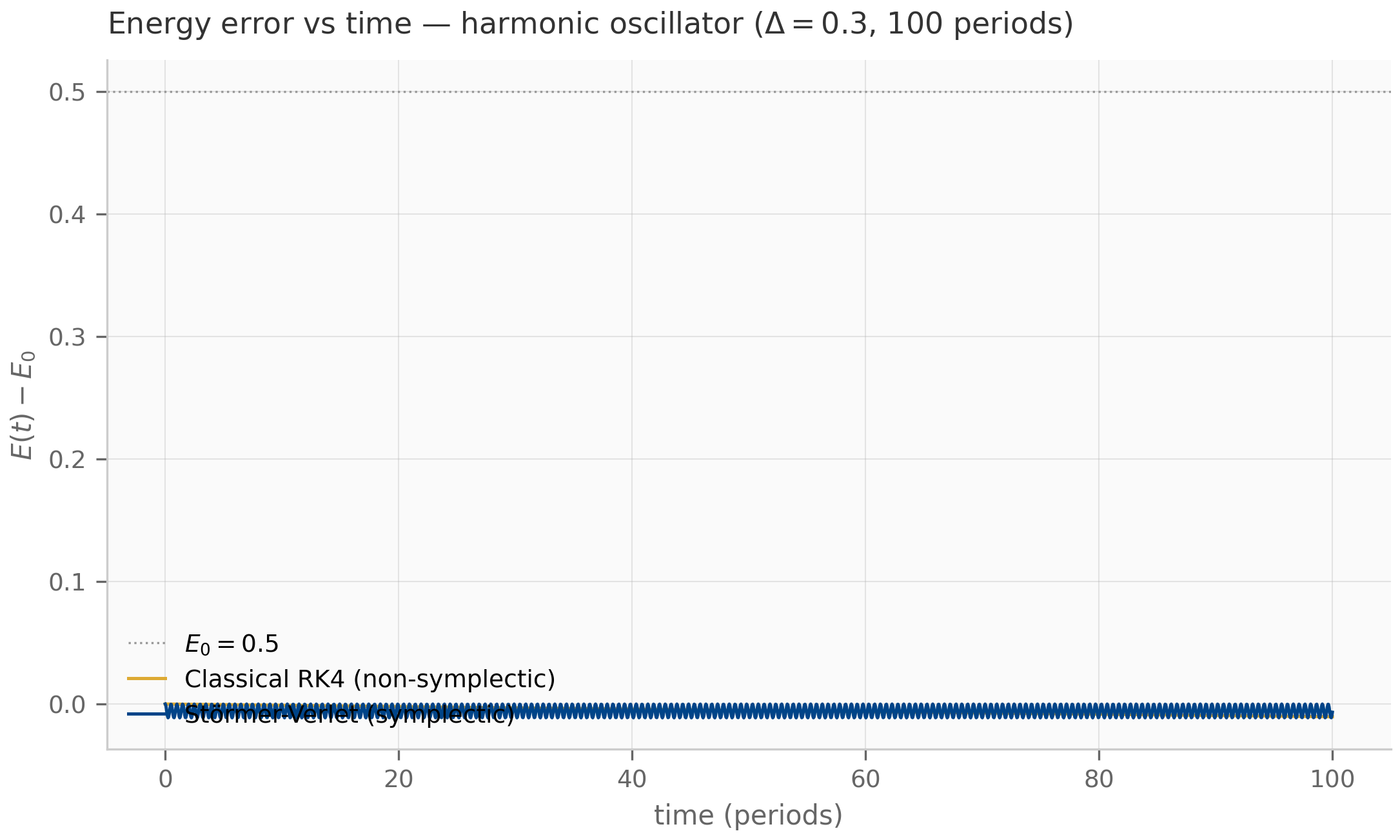
(Modified Hamiltonian for symplectic methods.) Let be a symplectic integrator of order applied to a system with analytic Hamiltonian , and let the step size satisfy for a problem-dependent threshold . Then there is a modified Hamiltonian whose optimally truncated partial sum is preserved along the discrete trajectory up to an exponentially small error over exponentially long times . The original therefore oscillates within a bounded band along the discrete trajectory.
The proof — Hairer–Lubich–Wanner Chapter IX — uses backward error analysis to expand the modified Hamiltonian as an asymptotic series in and shows the series can be truncated with controlled remainder. The takeaway for practice: a -th order symplectic integrator is exponentially better than a -th order non-symplectic one on Hamiltonian problems, even though the local truncation error of both is . Local error is misleading for long-horizon problems; geometric structure is what matters.
6.6 Toward selective SSMs as Hamiltonian flows
The C1 niche pilot proposes the following research program. The hidden-state dynamics of a selective SSM can sometimes be written as a Hamiltonian flow on the hidden-state manifold; when they can, applying a symplectic integrator should reduce long-horizon error in a way that order-optimized integrators cannot match. The first step is to characterize when this Hamiltonian structure exists.
For a linear-time-invariant SSM , the dynamics are Hamiltonian iff there exists a symmetric positive-definite such that . Equivalently, is similar (via ) to a skew-symmetric matrix. The quadratic Hamiltonian is then , and the symplectic 2-form is (in the standard symplectic-flat coordinates). For HiPPO-LegS the eigenvalues are all real-negative, not purely imaginary, so HiPPO-LegS dynamics are dissipative, not Hamiltonian. Symplectic methods do not apply. This is consistent with the empirical observation that ZOH and bilinear discretizations of HiPPO-LegS perform well — dissipation handles the long-horizon stability story.
For a selective SSM with input-dependent , the relevant question becomes: does have a Hamiltonian decomposition for some range of inputs, even if not for all? The C1 pilot’s empirical hypothesis is that during certain training phases the learned matrices drift toward eigenvalue spectra that are closer to purely imaginary than to the LHP, and that this drift is associated with the long-horizon recall artifacts observed in Mamba’s failure modes Halloran et al. (2025) . If this hypothesis holds, then symplectic discretization of selective SSMs should reduce those artifacts. The Chapter 17 pilot integration develops this thread; this chapter has supplied the necessary integration-theory vocabulary.
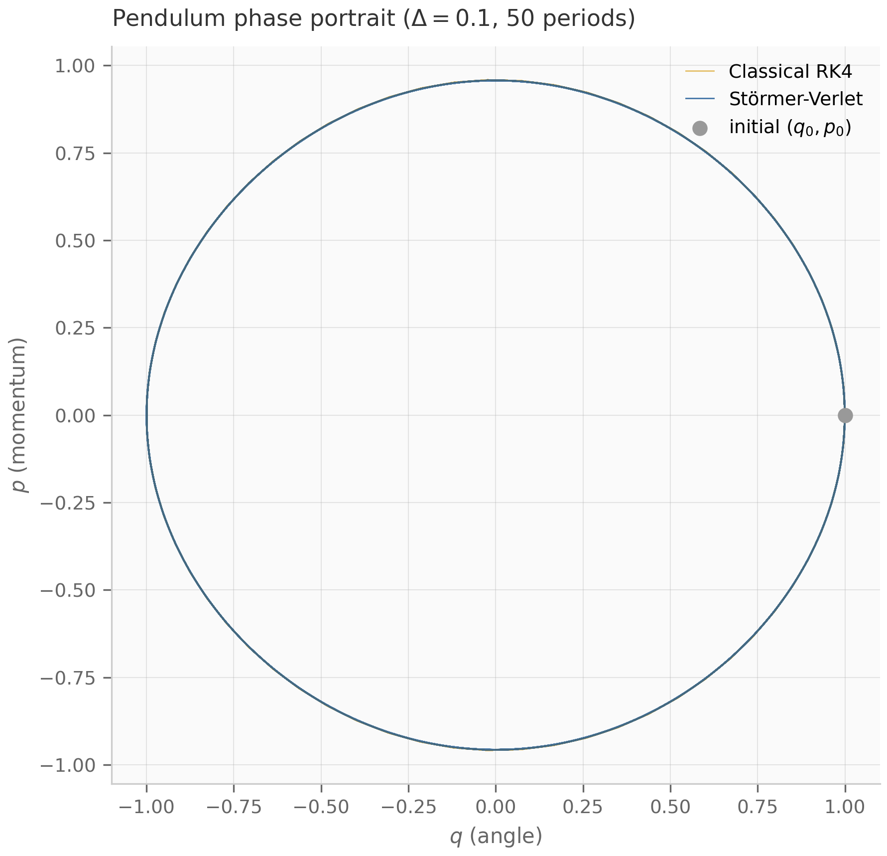
6.7 What’s next
This chapter completes the foundations layer of the book (Part I). The next part — Chapters 7–10 — introduces structured SSMs (S4, S4D, S5, Mamba-1/2, Mamba-3) as discretizations of the continuous systems developed here. Chapter 7 sets up HiPPO theory; Chapter 8 derives the S4 / S4D / S5 architectures (and sorts out which discretization each paper actually used); Chapter 9 introduces selective scans (Mamba-1/2); Chapter 10 brings the exp-trapezoidal scheme of §4.5 to its home in Mamba-3.
The C1 pilot integration in Chapter 17 returns to this chapter’s symplectic story, applying the modified-Hamiltonian framework to learned selective dynamics. Readers focused on the SSM applications can skip to Chapter 7 now and consult §6.5–§6.6 when the symplectic discussion comes back.
6.8 Exercises
Six problems. Short/numerical (6.1–6.3) have inline collapsible solutions; long/proof exercises (6.4–6.6) have full worked solutions in §6.9.
Exercise 6.1 (computation)
Verify that backward Euler’s stability function is by directly applying the scheme to the test problem and solving for .
Solution
Backward Euler: . Rearranging, , so . Setting , the stability function is . ∎
Exercise 6.2 (computation)
For the harmonic oscillator , (so ), compute one step of symplectic Euler (“p first” variant) starting from at . What are , and what is ?
Solution
Symplectic Euler ( first): , then .
Starting from : . Then . So .
Energy: . Initial energy was . The energy is not exactly preserved (it changed by ), but it is bounded — over many steps it will oscillate, not drift.
Exercise 6.3 (computation + code)
Run companions/ch06/jax/symplectic_demo.py. Verify that classical RK4 produces linear-in-time energy drift on the harmonic oscillator while Störmer–Verlet’s energy stays in a bounded band. What is the drift rate (energy per period) of RK4 at ?
Solution
The companion’s main output shows two energy-vs-time traces over 100 periods. RK4 drifts approximately linearly; the drift rate at is roughly per period — small in absolute terms but growing linearly with horizon (so ~ after 100 periods, ~ after 1000). The linear-time growth rate, not the absolute magnitude, is the diagnostic. Störmer–Verlet’s energy stays within a bounded band of width , with no secular drift no matter how long the run. The contrast — monotonic linear-in-time growth vs bounded oscillation — is the key takeaway of §6.5, and is the horizon-invariance of the symplectic band rather than the absolute magnitude at any specific that defines a symplectic method.
Exercise 6.4 (theory) — solution in §6.9
Prove the L-stability of backward Euler (Proposition 6.1): for , and as .
Exercise 6.5 (theory) — solution in §6.9
Show that symplectic Euler is symplectic. That is, prove that the Jacobian has determinant exactly 1 for the harmonic oscillator. (Then note: for separable Hamiltonians, the same argument applies via the chain rule.)
Exercise 6.6 (theory) — solution in §6.9
Show that for a linear-time-invariant ODE with skew-symmetric (), the function is a constant of motion. Use this to give a sufficient condition (in terms of only) for an SSM to be Hamiltonian.
6.9 Full solutions to theory exercises
Solution to Exercise 6.4
Write with . Then . Since , , so . Therefore . ∎
For the L-stability limit: as with bounded, , so . ∎
Solution to Exercise 6.5
For the harmonic oscillator , , symplectic Euler ( first) gives
The Jacobian is
The determinant: . ∎
So the discrete map preserves the symplectic 2-form exactly. This is the algebraic content of “symplectic Euler is symplectic” — the determinant being exactly , not .
For a general separable Hamiltonian , symplectic Euler gives and . The Jacobian factorizes as
each of which has determinant 1 (lower- and upper-triangular with 1s on the diagonal). The product determinant is therefore 1. ∎
This “shear-decomposition” argument generalizes to all symplectic integrators that update and in alternating steps: each individual sub-step is a shear, with unit determinant. Verlet, leapfrog, Yoshida composition methods — all are products of unit-determinant shears.
Solution to Exercise 6.6
For with , compute
since by skew-symmetry. So — the squared norm is exactly preserved. ∎
Sufficient condition for an SSM to be Hamiltonian. Any SSM whose continuous dynamics matrix is skew-symmetric is Hamiltonian with Hamiltonian . The eigenvalues of a real skew-symmetric matrix are purely imaginary (or zero), so this regime is exactly the purely oscillatory corner of the SSM landscape — the opposite of the LHP-stable corner where HiPPO and S4 live. A more general sufficient condition: has a Hamiltonian structure (in the matrix-Lie-algebra sense) — equivalently, there exists a symmetric positive-definite with . The C1 pilot’s empirical project is to identify selective-SSM regimes where this condition holds approximately, and to apply symplectic discretization there.
6.10 Companion code
Two JAX companions, two PyTorch companions, and two Julia companions for Chapter 6.
JAX (companions/ch06/jax/):
stiff_demo.py— van der Pol oscillator at (mildly stiff); compares explicit RK4 (blows up at large ) against backward Euler (stable at every ); emitsstiff_blowup.png.symplectic_demo.py— harmonic oscillator + pendulum; runs classical RK4 vs Störmer–Verlet over 100 periods; emitsenergy_drift.pngandphase_portrait.png.
Julia (companions/ch06/julia/):
implicit_methods.jl— backward Euler, BDF2, and DIRK from-scratch implementations on a stiff test problem; uses onlyLinearAlgebra+Printf.symplectic_methods.jl— symplectic Euler, Störmer–Verlet, and the 2-stage Gauss–Legendre IRK method on a Hamiltonian test; emits empirical order-of-accuracy table.Project.toml/Manifest.toml.
PyTorch (companions/ch06/torch/):
stiff_demo.py— the van der Pol RHS/Jacobian with RK4 and backward-Euler steppers (compute-only; the JAX companion produces the figure).symplectic_demo.py— the RK4 and Störmer–Verlet steppers on the harmonic oscillator and pendulum.tests/— cross-framework parity: the torch trajectories and energy-drift quantities equal their JAX counterparts to within (float64).
To run from the repo root:
# JAX
PYTHONPATH=. python companions/ch06/jax/stiff_demo.py
PYTHONPATH=. python companions/ch06/jax/symplectic_demo.py
# PyTorch (needs the .venv [torch] extra; parity only, no figures)
PYTHONPATH=. python companions/ch06/torch/stiff_demo.py
PYTHONPATH=. python companions/ch06/torch/symplectic_demo.py
# Julia (lightweight — no DifferentialEquations.jl dependency)
julia --project=companions/ch06/julia companions/ch06/julia/implicit_methods.jl
julia --project=companions/ch06/julia companions/ch06/julia/symplectic_methods.jlAll figures emit to public/figures/ch06/.
HiPPO theory: orthogonal-basis projection operators
Online function approximation by projection onto orthogonal polynomial bases — the HiPPO-LegS operator, its lower-triangular structure and exact spectrum, discretization to the S4 recurrence, and the basis-conditioning question.
HiPPO theory: orthogonal-basis projection operators
7.1 The online function-approximation problem
A recurrent model carries a finite state and updates it one sample at a time. The central question is what should that state store? HiPPO’s answer is sharp: the state should store a compressed representation of the entire input history, chosen so that the history can be reconstructed as accurately as numbers allow.
Make this precise. Fix a time and consider the input seen so far, for . Equip the interval with a measure (a weighting that says which parts of the history matter). The best -term approximation of in the weighted space is its orthogonal projection onto an -dimensional subspace spanned by basis functions :
The coefficient vector is the compressed memory. HiPPO’s discovery is that for well-chosen bases obeys a linear ODE in — so maintaining the optimal projection online is exactly running a linear state-space model.
The picture to keep in mind is reconstruction. Drive a signal into the operator, read off at the final time, and expand : you recover the history, and the recovery sharpens as grows. 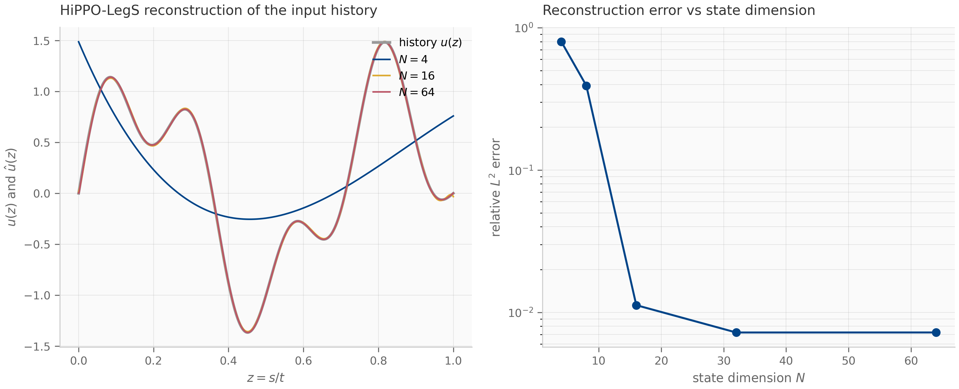
7.2 Orthogonal polynomial bases
The natural basis for functions on an interval is the Legendre polynomials . On they are orthogonal under the uniform measure,
and satisfy the three-term recurrence with , . Rescaling to the unit interval and normalizing gives an orthonormal family
These are the basis functions HiPPO projects onto; the companion’s Gram-matrix check confirms their orthonormality to under trapezoidal quadrature. 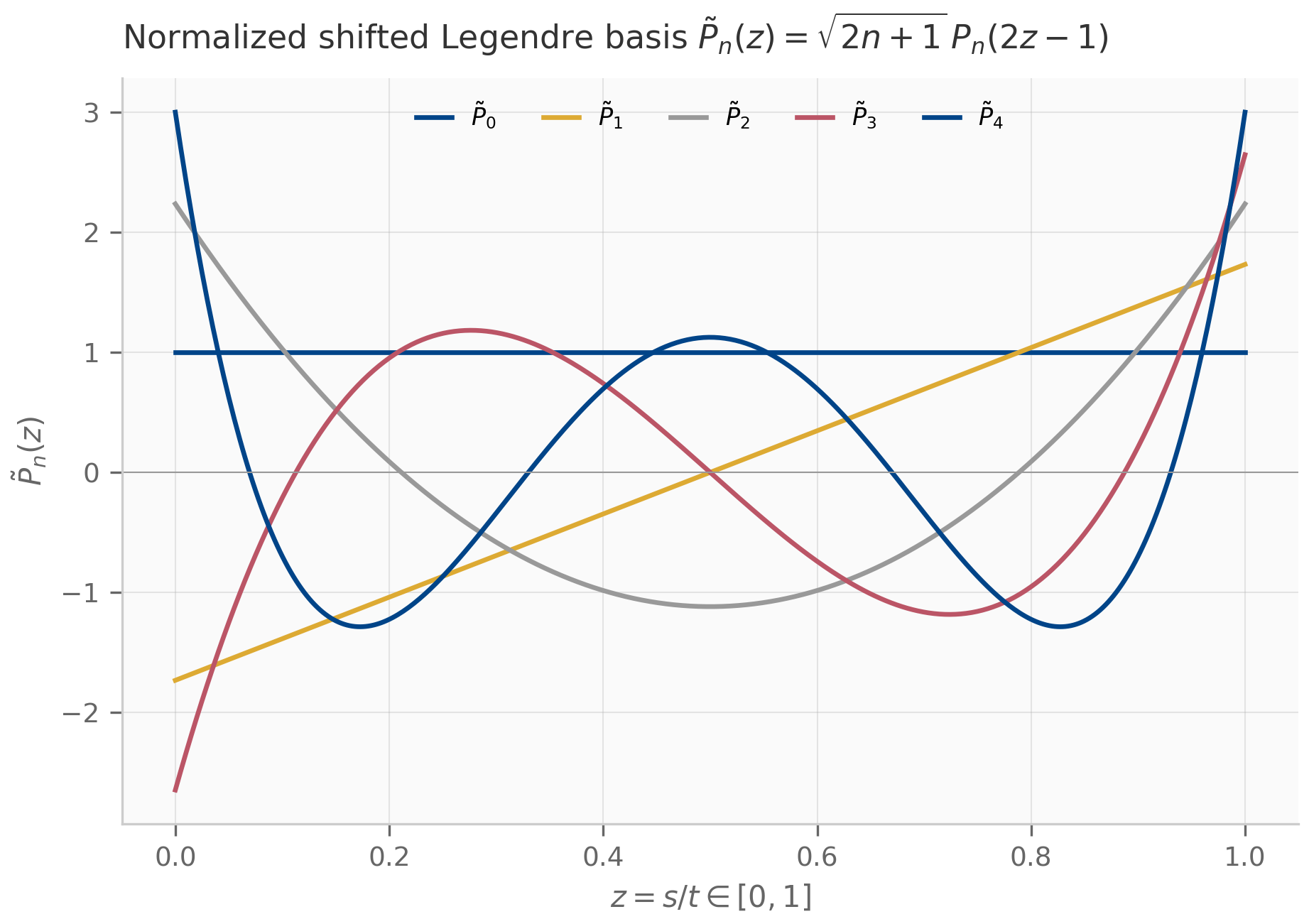
Orthogonality is what makes projection cheap and optimal. Because the basis is orthonormal, the best approximation is obtained coefficient-by-coefficient — no linear system to solve.
(Orthogonal projection is the best approximation.) Let be orthonormal in and let . For any , the coefficients minimize the reconstruction error: for every , with equality only when .
The proof (Exercise 7.5, §7.10) is the Hilbert-space Pythagorean theorem: the residual is orthogonal to , so any other only adds an orthogonal error that grows the norm.
The measure encodes which history matters. Two choices dominate the HiPPO literature Gu et al. (2020) :
- LegT (translated Legendre): a sliding window of fixed length — the state remembers the most recent time units uniformly and forgets everything older. This is a fixed-horizon memory.
- LegS (scaled Legendre): the growing window with uniform weight, rescaled as increases. The state remembers all history, allocating its coefficients to the whole past at every scale. This is the variant that gives S4 its long-range reach, and the one we develop in detail.
7.3 The HiPPO-LegS operator
For the scaled measure the projection coefficients obey a strikingly clean ODE. Differentiating through the time-dependence of the measure and using the Legendre recurrence yields the HiPPO-LegS dynamics, a linear state-space system whose matrices have a closed form.
(HiPPO-LegS closed form.) The scaled-Legendre projection coefficients evolve under a linear system with state matrix and input matrix given by
for . In particular is lower-triangular.
The derivation (Exercise 7.4, §7.10) substitutes the Legendre three-term recurrence into the time-derivative of the projection integral; the lower-triangular structure is inherited from the recurrence, which expresses using only lower-degree polynomials. The matrix has a vivid signature: a negative diagonal that grows linearly, and negative off-diagonal entries below it that grow like .
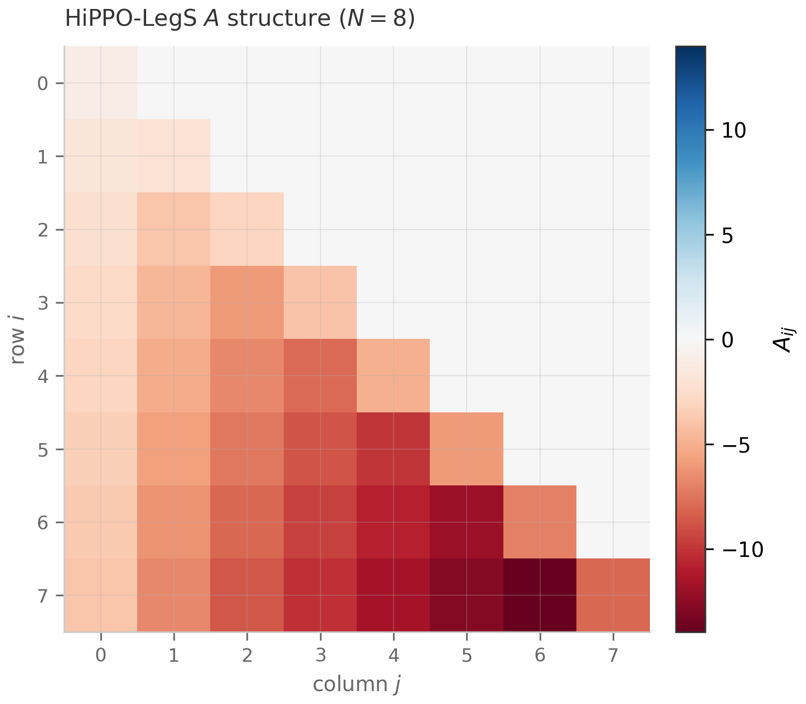
This is the answer to Chapter 4’s open question. Where Chapter 4 asked “given , how do we discretize it?”, HiPPO supplies the — not by guessing, but as the projection-update operator of an optimal polynomial memory. Random initialization of produces eigenvalues scattered across the complex plane and dynamics that vanish or explode over long horizons; the HiPPO is engineered so that its discretization gives stable, long-memory recurrences Gu et al. (2020) .
7.4 From the operator to the S4-style recurrence
To run the HiPPO operator on sampled data we discretize the LTI system exactly as in Chapter 4 §4.3. The zero-order hold gives
computed in practice through the augmented matrix-exponential trick of Chapter 4 (the HiPPO is invertible — that promise from §4.3 is kept here). Because every eigenvalue of has negative real part (§7.7), Chapter 4’s ZOH stability proposition applies verbatim: every discrete eigenvalue satisfies , so the recurrence is stable for any step size. ZOH is this book’s default discretization throughout Chapters 7–9 precisely because it preserves the HiPPO spectrum so cleanly (the original S4 paper used the bilinear transform instead, and S4D supports either; Chapter 4 §4.6 lays out the trade-off).
This recurrence is the recurrent view of an S4-style layer Gu et al. (2022) . Chapter 8 adds the second view — unrolling the recurrence into a convolution and computing it with an FFT — and shows the two views are identical for zero initial state. The HiPPO matrix is exactly the initialization that S4 places on before training; S4D Gu et al. (2022) then diagonalizes it for speed, a move §7.5 explains is delicate precisely because of conditioning. Everything S4 does is downstream of the operator in §7.3.
7.5 Conditioning of the HiPPO basis
The HiPPO-LegS matrix is lower-triangular and its eigenvalues are the well-separated integers (§7.7), which sounds maximally benign. It is not, and the reason is non-normality: is far from symmetric, so its eigenvectors are highly oblique and the matrix that diagonalizes it is ill-conditioned. The condition number of that eigenvector basis grows exponentially in Yu et al. (2023) , so a naive diagonalization of HiPPO-LegS is numerically untrustworthy at the used in practice — and the sub-quadratic conditioning one wants is achieved only by deliberately perturbing the transform (the “robustifying” construction below).
Two consequences follow. First, diagonalization is dangerous: S4D’s diagonal reparameterization Gu et al. (2022) must be done in a numerically careful (often complex, approximately-diagonal) form, and the “robustifying” line of work Yu et al. (2023) exists exactly to tame the conditioning of the diagonalizing transform. Second, the choice of discretization interacts with conditioning: a poorly conditioned basis amplifies the per-step error of a low-order scheme, so the second-order schemes of Chapter 4 (and the geometric integrators of Chapter 6) are not academic refinements but a response to a real failure mode. This conditioning question is the seed of research niche C4 — characterizing where HiPPO-style projections become numerically untrustworthy and what to do about it.
7.6 Alternative bases
Legendre is one choice among many; HiPPO is a framework parameterized by the basis–measure pair Gu et al. (2023) . Swapping the basis changes what the state is good at remembering:
- LagT (Laguerre): an exponentially-weighted infinite horizon — the measure decays into the past, so the state emphasizes recent history with a graceful tail.
- FouT (Fourier): a Fourier basis on a sliding window, well matched to periodic or oscillatory inputs; closely related to the implicit long convolutions of Chapter 11.
- Wavelet bases (WaLRUS): replacing polynomials with a redundant wavelet frame Babaei et al. (2025) shifts the optimal-projection target from polynomial smoothness to wavelet sparsity, which can suit signals with localized or multi-scale structure better than a global polynomial basis.
The “How to Train Your HiPPO” generalization Gu et al. (2023) derives the projection ODE for arbitrary measure–basis pairs and identifies which ones are well-conditioned to train — directly connecting basis choice back to §7.5. The lesson is that the structure of (lower-triangular, stable spectrum, projection-update semantics) survives the basis change; the closed-form entries do not. When a later chapter reaches for a non-Legendre SSM, this is the machinery underneath.
7.7 Eigenvalue structure and stability
Return to the matrix itself. Because is lower-triangular, its eigenvalues are exactly its diagonal entries.
(HiPPO-LegS spectrum.) The eigenvalues of the HiPPO-LegS matrix are exactly — real, distinct, and strictly negative. Consequently the continuous system is asymptotically stable (Chapter 2), and its ZOH discretization has all discrete eigenvalues strictly inside the unit disk for every (Chapter 4).
The proof is immediate from lower-triangularity (Exercise 7.6, §7.10). The companion verifies it numerically: for up to the computed eigenvalues match to better than , and the strict upper triangle is exactly zero. 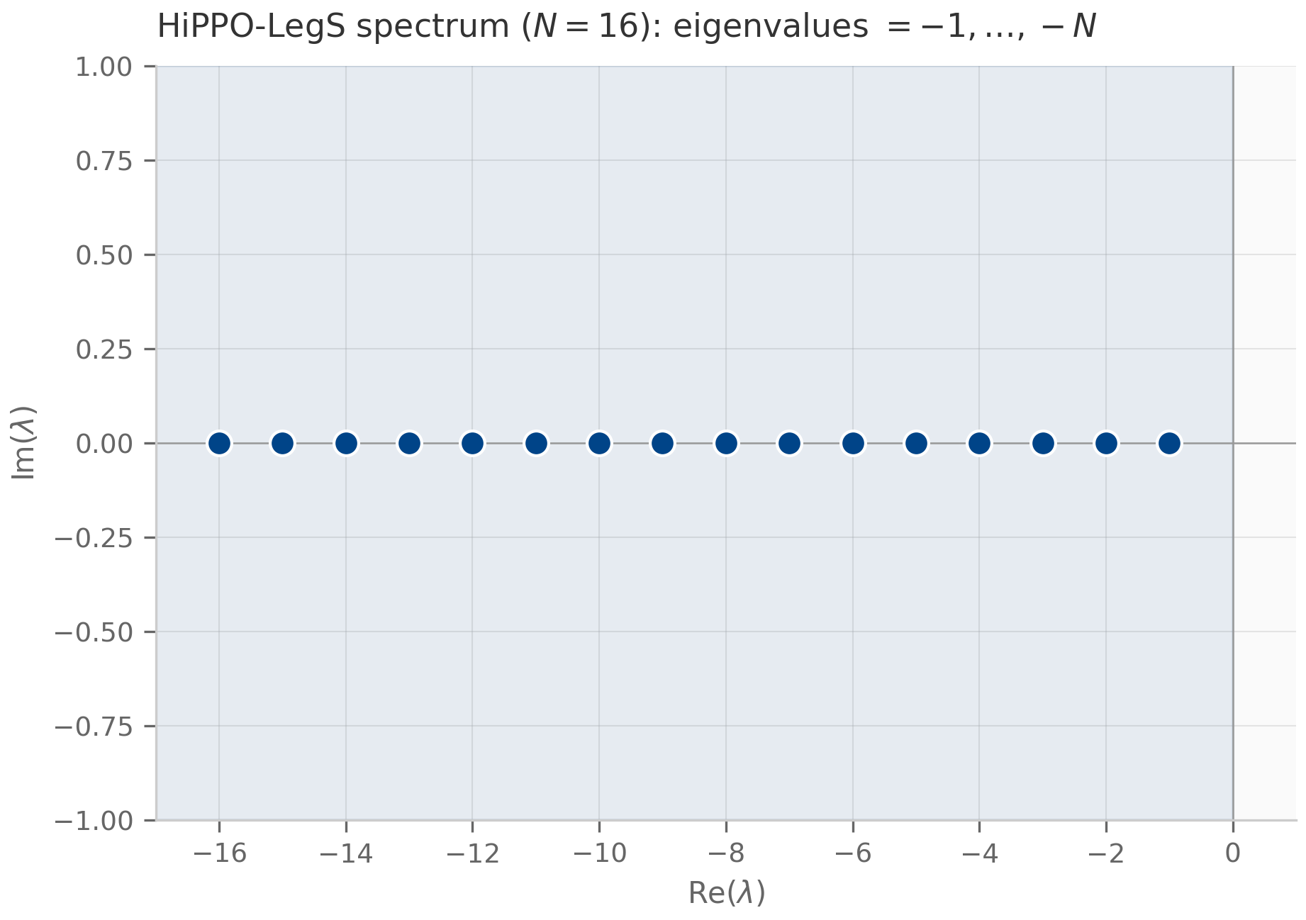
The integer spectrum has a memory interpretation: under ZOH the -th mode decays per step by , so low-index coefficients (coarse features of the history) are long-lived while high-index coefficients (fine detail) fade fastest. The state is a graded, multi-timescale memory — and the learnable slides the whole schedule. This is the dynamical-systems reading of why HiPPO works, and it is the structure a stability or Lyapunov analysis of a trained S4 layer (Chapter 15) measures against.
7.8 What’s next
This chapter answered “what is ?” with “the projection-update operator of an optimal polynomial memory,” and showed that operator is lower-triangular, stably-spectrumed, and ZOH-discretizable into a recurrence. Chapter 8 takes that recurrence and develops the full S4 / S4D / S5 machinery: the convolutional view, the FFT kernel, the diagonalization that §7.5 warned is delicate, and the parallel scan. Chapter 9 then makes the parameters input-dependent — the selective SSMs (Mamba) — and Chapter 10 swaps ZOH for the exponential-trapezoidal scheme of Chapter 4 when the dynamics turn stiff. HiPPO is the hinge: every architecture from here inherits the structured derived in §7.3.
7.9 Exercises
Six problems mixing computation and theory. Short/numerical (7.1–7.3) have inline collapsible solutions; the theory exercises (7.4–7.6) have full worked solutions in §7.10.
Exercise 7.1 (computation)
Using the three-term recurrence, write down and verify by direct integration that . Then confirm .
Solution
. The product is even, and , so the integral is — Legendre orthogonality. For the norm, , matching .
Exercise 7.2 (computation)
Build the HiPPO-LegS matrix from the closed form of §7.3 by hand. Verify that and that the diagonal is .
Solution
Entry has , so . The diagonal entries are for , i.e. . The full matrix is lower-triangular with , and zeros above the diagonal. The companion hippo_matrix.py prints exactly .
Exercise 7.3 (computation + code)
Run companions/ch07/jax/hippo_reconstruction.py. Confirm that the relative reconstruction error of the two-sinusoid test signal falls sharply from to , then plateaus. Why does it plateau rather than continue to zero?
Solution
The companion prints errors . The sharp drop happens once is large enough to represent the signal’s two frequencies (≈ 1.5 and 4 cycles on the window); beyond that the error plateaus at the discretization floor of the time-varying LegS recurrence at the chosen sample count (), not at zero. Adding more Legendre modes cannot beat the error already incurred by integrating the projection ODE on a finite grid — exactly the conditioning/discretization interaction of §7.5. The Julia and PyTorch companions reproduce these numbers to machine precision.
Exercise 7.4 (theory) — solution in §7.10
Show that the HiPPO-LegS matrix is lower-triangular, and that its diagonal entries are , by appealing to the structure of the Legendre three-term recurrence. (You may take the off-diagonal closed form as given; the point is the structure.)
Exercise 7.5 (theory) — solution in §7.10
Prove the best-approximation theorem (Theorem, §7.2): if is orthonormal in and , then is the unique minimizer of over .
Exercise 7.6 (theory) — solution in §7.10
Using lower-triangularity, prove that the eigenvalues of are exactly . Then show that ZOH discretization sends every eigenvalue strictly inside the unit disk for all , and identify the per-step decay rate of the -th mode.
7.10 Full solutions to theory exercises
Solution to Exercise 7.4
The shifted Legendre polynomials satisfy a three-term recurrence in which is expressed through and — never through higher-degree polynomials. When the projection coefficient is differentiated in , the time-derivative of the (scaled) measure couples to the inner products of against — and the recurrence guarantees only appear. Hence depends on but not on , which is exactly the statement that has zero entries above the diagonal: for . For the diagonal, the “self-coupling” term of the -th coefficient under the scaled measure contributes (the normalization and the measure’s scaling combine to the integer ); this is the claim. The off-diagonal entries for follow from the same expansion carried through the normalization, given here without the full bookkeeping.
Solution to Exercise 7.5
Let with , and let be any element of . First, the residual is orthogonal to every :
using orthonormality . Therefore , and in particular since . Now decompose and apply the Pythagorean theorem:
with equality iff , i.e. . So is the unique minimizer.
Solution to Exercise 7.6
A lower-triangular matrix has its eigenvalues on the diagonal: is the product of diagonal entries because the determinant of a triangular matrix is the product of its diagonal, and subtracting keeps it triangular. With the roots are for , i.e. exactly — real, distinct, strictly negative.
Under ZOH the discrete dynamics matrix is , whose eigenvalues are . Then
so every discrete eigenvalue lies strictly inside the unit disk (A-stability, Chapter 4). The per-step decay rate of mode is : higher-index modes decay faster, giving the graded multi-timescale memory of §7.7.
7.11 Companion code
Three runnable companions for Chapter 7 — the first SSM-core chapter, where the foundations and numerics threads meet in one operator. All three language tracks produce the same HiPPO-LegS matrix and the same reconstruction errors, which is itself the lesson: the mathematics is framework-independent; the idioms differ.
JAX (companions/ch07/jax/):
hippo_matrix.py— builds the HiPPO-LegS from the §7.3 closed form with a vectorizedjnp.where(no Python loop,jit-fusable); emitshippo_matrix_structure.pngandhippo_eigenvalues.png.hippo_reconstruction.py— runs the time-varying LegS recurrence viajax.lax.scanand reconstructs the history; emitslegendre_basis.pngandhippo_reconstruction.png.tests/test_hippo.py— pins the closed form, the integer spectrum, the reconstruction-error decay, and alax.scan-vs-naive-loop equivalence guard.
Julia (companions/ch07/julia/):
hippo_legendre.jl— the same operator with stdlibLinearAlgebraonly; the encoder is an explicitforloop (the contrast tolax.scan), and the Legendre basis is built from the three-term recurrence.runtests.jl—@testsetassertions including an orthonormality Gram-matrix check.
PyTorch (companions/ch07/torch/):
hippo_operator.py— HiPPO-LegS wrapped as annn.Moduleprojection operator (fixed buffers, zero learnable parameters); a define-by-run eager loop encodes the signal. This is the object Chapter 8’s S4 layer extends.tests/test_hippo_torch.py— cross-framework consistency: the matrix matches the closed form and the reconstruction errors reproduce the JAX/Julia numbers.
To run from the repo root:
# JAX (uses the uv .venv with jax, numpy, scipy, matplotlib)
PYTHONPATH=. python companions/ch07/jax/hippo_matrix.py
PYTHONPATH=. python companions/ch07/jax/hippo_reconstruction.py
# Julia (stdlib only; instantiates instantly)
julia --project=companions/ch07/julia companions/ch07/julia/hippo_legendre.jl
# PyTorch (needs the .venv [torch] extra)
PYTHONPATH=. python companions/ch07/torch/hippo_operator.pyAll figures emit to public/figures/ch07/.
LTI SSMs: S4, S4D, S5 as discretized continuous systems
The S4 architecture as a discretized HiPPO LTI system — the convolution–recurrence duality and its FFT kernel, the diagonal-plus-low-rank structure behind S4's fast kernel, S4D's diagonal restriction with by-construction stability, and S5's parallel associative scan.
LTI SSMs: S4, S4D, S5 as discretized continuous systems
8.1 State-space to discrete: the S4 setup
Chapter 7 closed on a recurrence and called it the recurrent view of an S4-style layer. Make the layer explicit. S4 fixes a single-input, single-output (SISO) continuous system
with the HiPPO-LegS matrix of §7.3, , , and a scalar feedthrough. To run it on a sampled sequence we discretize at step . The S4 paper itself uses Chapter 4’s bilinear transform (§4.4), Gu et al. (2022) ; this book standardizes on the zero-order hold (§4.3) — the rule S5 Smith et al. (2023) and the Mamba line Gu & Dao (2024) later adopted, and one whose difference from bilinear the S4D ablations measure as negligible Gu et al. (2022) :
computed through the augmented matrix-exponential trick of §4.3 (the companion’s discretize_zoh stacks and exponentiates, sidestepping ).
What makes this an architecture rather than a fixed filter is which parts train. S4 learns , , and (the timescale, kept positive by the log), while are initialized from HiPPO and often frozen or updated slowly. Stability is inherited for free: by the §7.7 spectrum every eigenvalue of has negative real part, so Chapter 4’s ZOH proposition gives for every . The slowest mode (eigenvalue ) decays per step by — for the companion’s default that is , a long but strictly contracting memory.
This is one way to compute the layer. The rest of the chapter is, in large part, other ways to compute the same thing — and the surprising fact that they are equal.
8.2 The structured state matrix, revisited
Before the second view, recall why the HiPPO is special enough to deserve fast algorithms. It is dense and lower-triangular (§7.3), so a black-box and a black-box kernel would cost more than the structure warrants. The structure S4 exploits is that the HiPPO-LegS matrix is normal-plus-low-rank (NPLR): up to an orthogonal change of basis it is a normal matrix plus a rank-one correction, and after diagonalizing the normal part it becomes diagonal-plus-low-rank (DPLR),
with the (complex) diagonal of eigenvalues and a rank-one term Gu et al. (2022) . That the HiPPO-LegS matrix admits this diagonal-plus-rank-one form is not evident from the §7.3 closed form — it is a construction of the S4 paper, which we take as given rather than re-derive here. This is the same non-normality that §7.5 flagged as a conditioning hazard, now read constructively: the eigenvector basis is oblique (hence ill-conditioned), but the correction that makes non-normal is only rank one, and a rank-one correction is exactly what the Woodbury identity handles cheaply.
The DPLR form is the hinge for the rest of the chapter. Section 8.4 uses the full to compute S4’s kernel quickly; §8.5 throws away the term entirely and keeps only , which is S4D.
8.3 The convolution–recurrence duality
The recurrence of §8.1 is sequential: needs . Unrolling it from zero initial state exposes a second, fully parallel description. With ,
Define the SSM convolution kernel by . Then the output is a causal convolution plus the feedthrough:
(Convolution–recurrence duality.) For zero initial state, the SISO recurrence , produces exactly the convolution with kernel , . The recurrent form costs sequential steps; the convolution, computed by FFT, costs parallel work.
The proof (Exercise 8.4, §8.9) is the unrolling above made rigorous by induction. The two forms are not approximations of each other — they are the same numbers. The companion confirms it to machine precision: the recurrent lax.scan output and the FFT convolution agree to a measured residual in float64, which test_conv_recurrence_duality pins below .
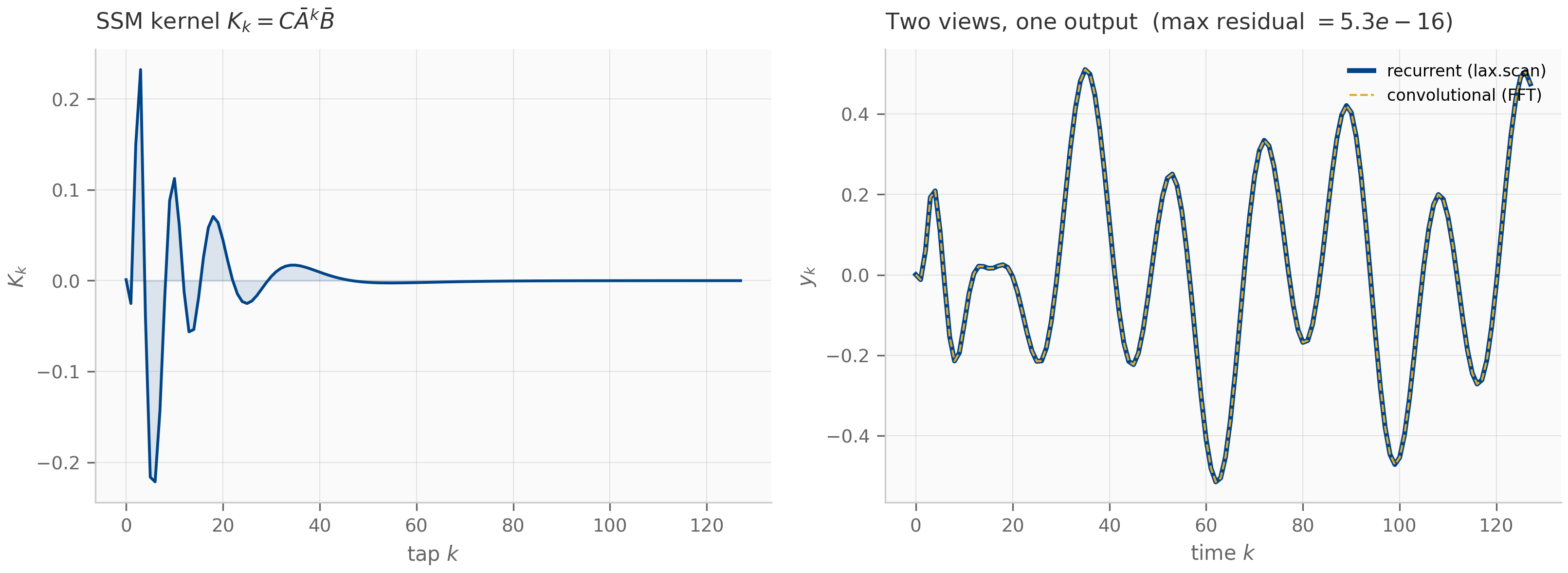
The duality is why S4 is practical: train as a convolution, deploy as a recurrence. Training sees whole sequences at once, so the parallel FFT wins; autoregressive inference produces one token at a time, so the scan with its state wins. One set of parameters, two runtimes.
8.4 The Cauchy kernel: structure buys speed
The duality leaves one cost open: building the kernel . Naively, iterates the state vector — one mat-vec per tap, in total. For the teaching regime that is exactly what the companion does, and it is plenty fast. S4’s published contribution is to compute the same kernel in near-linear time, , by using the DPLR structure of §8.2 Gu et al. (2022) .
The route is a generating function. Collect the taps into a polynomial and evaluate it on the unit circle: the truncated generating function is
a geometric series in the matrix . Recovering from evaluated at the -th roots of unity is one inverse FFT. The remaining cost is the resolvent , and here DPLR pays off: with built from the Woodbury identity turns the resolvent into a Cauchy matrix–vector product — entries — plus a rank-one correction. The whole kernel is then a Cauchy/Woodbury solve in plus the inverse FFT in (the §8.4 figure isolates the -scaling at fixed ); the dense never appears.
We present this kernel but do not implement it: the companions use the transparent naive kernel throughout (§8.10). The point of §8.4 is the shape of the cost, not the engineering — and the shape is what motivates S4D.
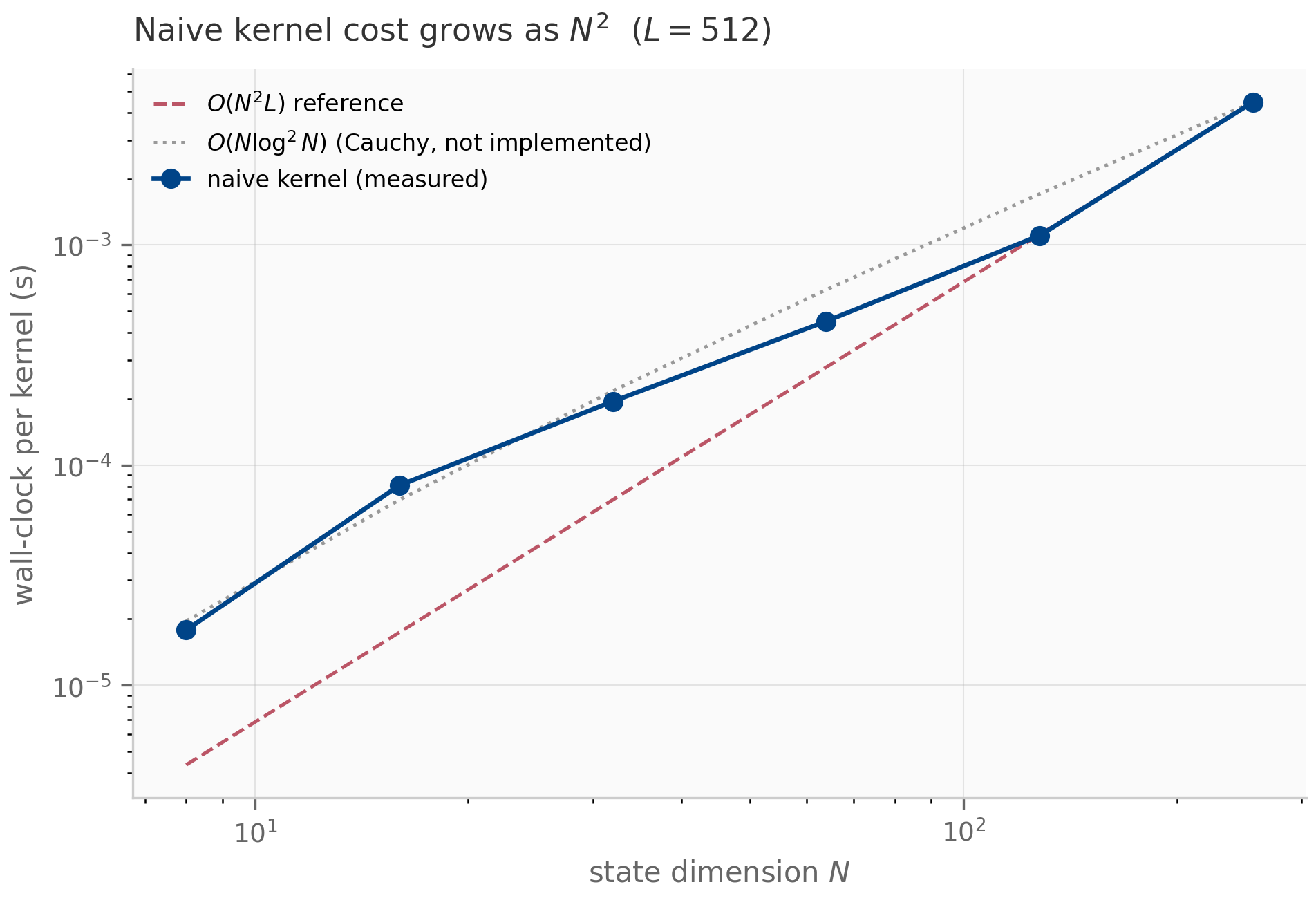
8.5 S4D: the diagonal restriction
The Cauchy machinery is the price of keeping the rank-one term . S4D asks what happens if we simply drop it Gu et al. (2022) — keep the diagonal , discard the low-rank correction. The state matrix is now genuinely diagonal, , and everything decouples mode by mode. The kernel collapses from a Cauchy computation to a Vandermonde sum:
with the per-mode diagonal ZOH input (this book’s convention; the S4D paper itself treats the integration rule as interchangeable — its base version keeps S4’s bilinear — and measures no noticeable difference between the two). In practice the real states are carried as complex conjugate pairs and the real kernel is reconstructed as .
(S4D Vandermonde kernel and stability.) For diagonal the kernel is the Vandermonde sum with . The discrete system is stable — every — if and only if for all .
The derivation and the stability claim are Exercise 8.5 (§8.9). What makes S4D more than “S4 with worse expressivity” is how it secures the stability condition. The S4D-Lin initialization places the modes at , and — crucially — stores them in the parameterization
so that for any real value the parameters take. Stability is not hoped for; it is structural.
This is the constructive answer to the §7.5 conditioning hazard: where S4 must diagonalize an ill-conditioned non-normal matrix and hope the basis behaves, S4D never forms that basis at all — it parameterizes the eigenvalues directly and pins their real parts negative.
Diagonal state space models are not a downgrade in practice: with the right initialization they match full S4 on long-range benchmarks while being markedly simpler to implement Gupta et al. (2022) . The companion plots the S4D-Lin spectrum against the full HiPPO spectrum to make the restriction visible.
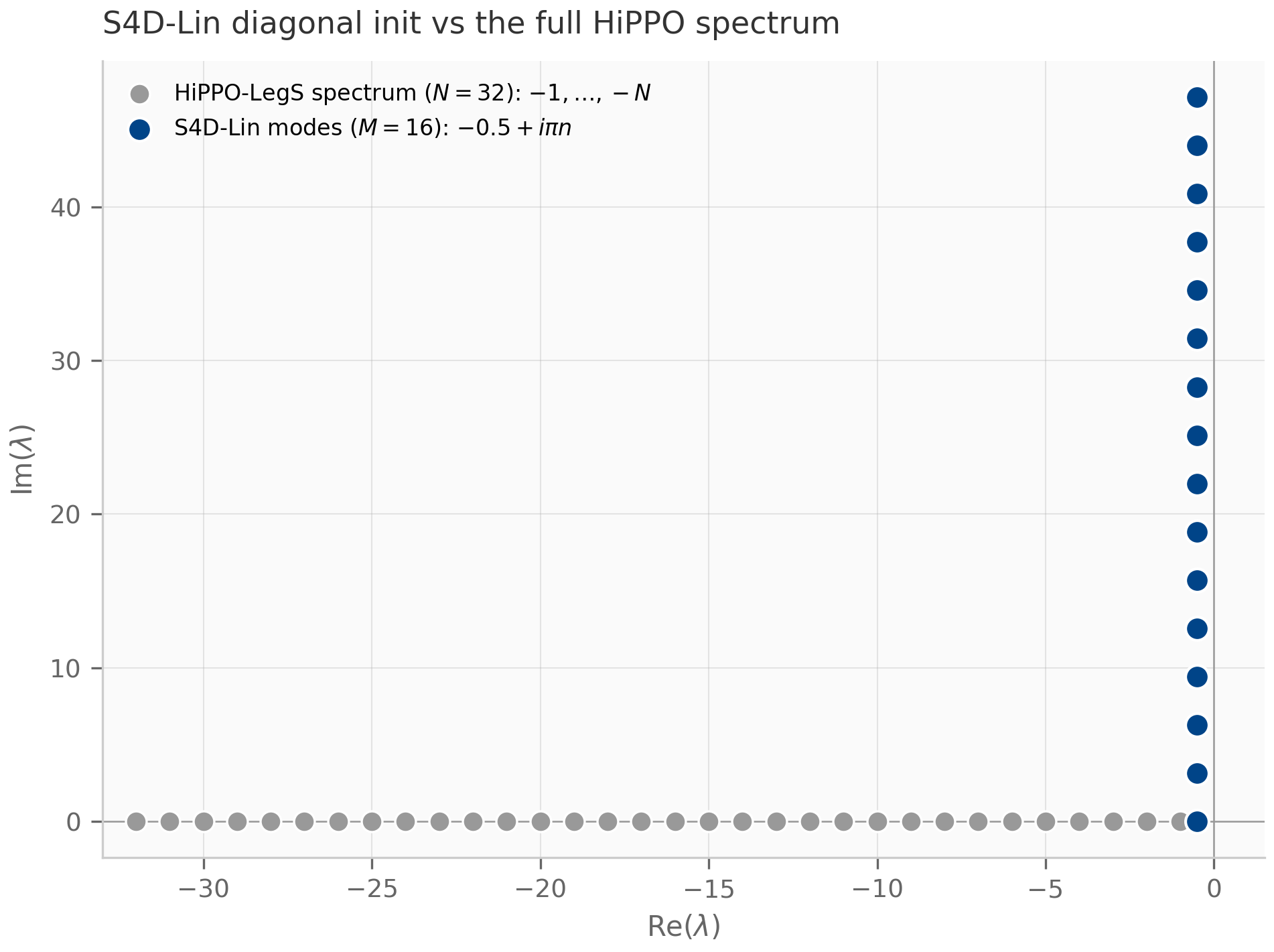
8.6 S5: the parallel associative scan
S4D made the state diagonal but still computed it as a convolution. S5 keeps the diagonal state and abandons the convolution for a parallel scan Smith et al. (2023) . Two changes. First, S5 is MIMO: one shared diagonal state of size drives input/output channels through and , instead of independent SISO systems. Second, it computes the recurrence
(diagonal , so is elementwise) with an associative scan. The trick is that a linear recurrence is an associative operation on pairs:
which composes “apply the first affine update, then the second.” Scanning over the pairs yields every state at once.
(Scan equivalence.) The operator above is associative, and the inclusive prefix scan of under has as its second components exactly the sequential states . A balanced reduction computes all prefixes in parallel depth Blelloch (1990) , versus the depth of the sequential recurrence.
The proof is Exercise 8.6 (§8.9). The companion pins the equivalence to machine precision — the associative scan and the sequential scan agree to about (pinned below ) — and contrasts the two on the algorithmic cost that actually differs: critical-path depth.
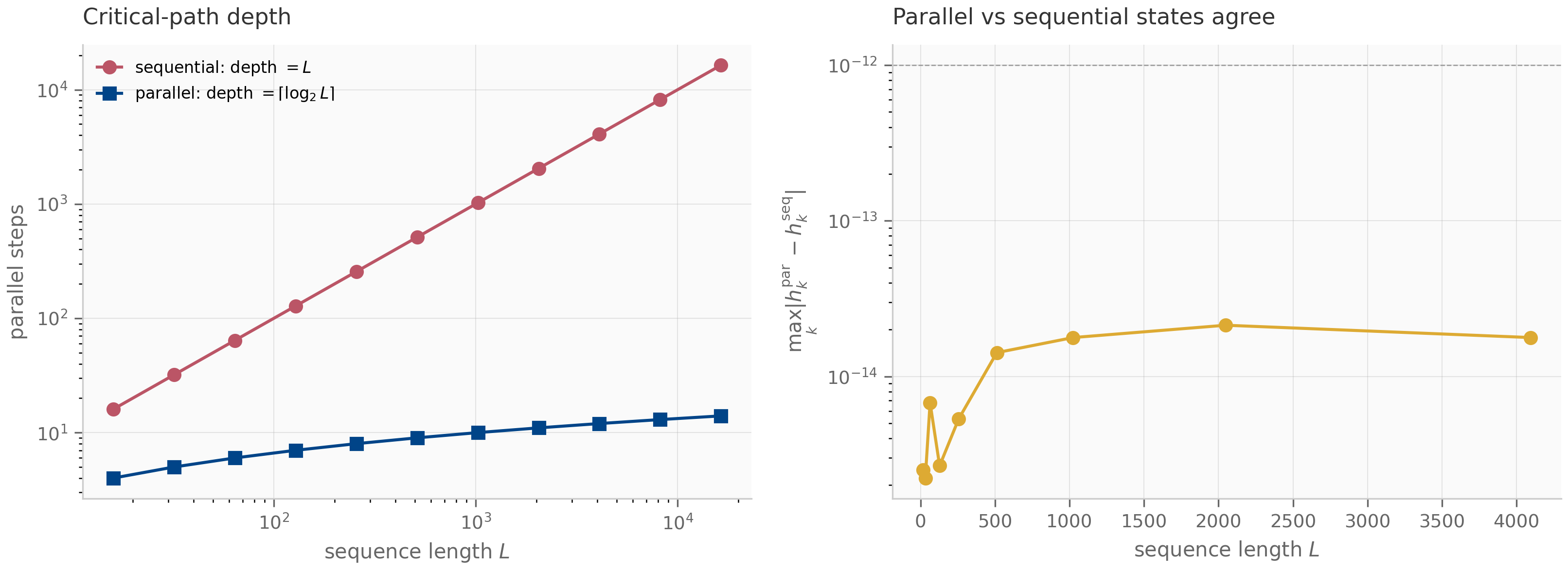
S5 deliberately stops at one diagonal SSM run in parallel. Its MIMO channel mixing and, above all, the move to input-dependent transitions are Chapter 9’s subject — and that move is what makes the associative scan indispensable rather than merely convenient.
8.7 What’s next
The thread of this chapter is that S4, S4D, and S5 are three computational treatments of one linear time-invariant system: a convolution and a recurrence that the duality proves equal (§8.3), a diagonal restriction whose stability is free (§8.5), and a parallel scan that reorders the same arithmetic into depth (§8.6). Time-invariance is what every one of these relies on — a fixed is what lets a single kernel exist and a single transition seed the scan.
Chapter 9 breaks time-invariance on purpose: Mamba makes functions of the input Gu & Dao (2024) (and the structured state-space duality Dao & Gu (2024) later reframes the result), which destroys the convolutional view and leaves the selective scan — the §8.6 primitive, now load-bearing — as the only way to compute the layer. Chapter 10 then replaces ZOH with the exponential-trapezoidal scheme of Chapter 4 when the selective dynamics turn stiff, in Mamba-3 Lahoti et al. (2026) ; that chapter is where the symplectic-integrator pilot finds its empirical anchor. Everything downstream inherits the discretized-LTI scaffold built here.
8.8 Exercises
Six problems mixing computation and theory. Short/numerical (8.1–8.3) have inline collapsible solutions; the theory exercises (8.4–8.6) have full worked solutions in §8.9.
Exercise 8.1 (computation)
Take a diagonal toy system , , , , and step . Compute and by the diagonal ZOH, then the first four kernel taps . Confirm the taps decay.
Solution
Diagonal ZOH acts mode-by-mode: and . So , and , . With the taps are :
Each tap is a sum of two decaying geometric sequences (rates and ), so the kernel decays monotonically — a discrete sum of exponentials, one per mode.
Exercise 8.2 (computation + code)
The S4D kernel sums one geometric sequence per mode. (a) Show that , so each mode decays at its own rate. (b) Show that a complex mode with weight and its conjugate with weight together contribute , explaining the real form. (c) Run companions/ch08/jax/s4d_kernel.py and confirm the Vandermonde kernel matches the recurrence oracle.
Solution
(a) , so and ; with this decays geometrically at rate per tap. (b) For any complex , since a number plus its conjugate is twice its real part; applying it with (and noting ) gives the claim. Carrying conjugate pairs and taking thus reproduces the -real-state kernel while storing only half as many complex numbers. (c) test_s4d_kernel_matches_recurrence_oracle pins the closed-form Vandermonde kernel against an independent complex-diagonal recurrence impulse response to .
Exercise 8.3 (code)
Run companions/ch08/jax/s4_duality.py and confirm the recurrent and convolutional outputs agree (the companion reports a residual below ). Then explain why the agreement would break if the FFT used length instead of .
Solution
The FFT computes a circular convolution of length equal to the transform size. With a length- transform, output position receives a contribution from kernel tap wrapped around the end of the sequence — a spurious term that the causal linear convolution does not contain, corrupting the early outputs. Zero-padding both signals to before the FFT makes the circular convolution agree with the causal linear one on the first positions (the wrapped terms land in the padded tail, which is discarded). The companion’s causal_conv_fft uses n = 2*L for exactly this reason; test_fft_pad_matches_direct_convolution pins the padded FFT against a direct convolution.
Exercise 8.4 (theory) — solution in §8.9
Prove the convolution–recurrence duality (Proposition, §8.3): for zero initial state, the SISO recurrence equals with .
Exercise 8.5 (theory) — solution in §8.9
Derive the S4D Vandermonde kernel from the diagonal recurrence, prove the discrete system is stable iff for all , and show that the S4D-Lin parameterization enforces stability for every parameter value.
Exercise 8.6 (theory) — solution in §8.9
Prove that the scan operator is associative, that its inclusive prefix scan reproduces the sequential states , and that a balanced reduction achieves parallel depth .
8.9 Full solutions to theory exercises
Solution to Exercise 8.4
Start from and . Claim: . Induct on . Base (): . Step: assuming ,
Now the output, using :
with . The sum is precisely the causal convolution , so . The lower-triangular Toeplitz structure of the map is the convolution.
Solution to Exercise 8.5
For diagonal the matrix exponential is diagonal, , and the ZOH input acts mode-by-mode: . The kernel inherits the diagonality,
a sum of geometric sequences — the Vandermonde form (the real version follows by pairing conjugates, Exercise 8.2). Stability: the kernel and the state stay bounded iff each geometric ratio satisfies . Since and , this holds iff for every . Finally, under S4D-Lin the real part is , and a negative exponential is strictly negative for every real exponent — so holds for all parameter values, with no constraint to enforce during training. Stability is built into the parameterization rather than maintained by it.
Solution to Exercise 8.6
Associativity. Write the action of a pair on a state as the affine map . Composition of affine maps is associative because function composition is. Concretely, with elementwise,
and the two right-hand sides are identical. Prefix scan reproduces the states. Let and be the inclusive scan. By induction the second component of equals : for it is (with ); and has second component . Depth. Because is associative, computing all prefixes is a prefix-sum problem, which a balanced binary reduction tree evaluates in sequential rounds with total work Blelloch (1990) — versus the rounds of the naive recurrence.
8.10 Companion code
Two language tracks for Chapter 8 — JAX (the reference, with the parallel scan) and PyTorch (the nn.Module operators). Julia is omitted here: the S4D reference and the associative-scan primitive both live in the JAX/PyTorch world, and a stdlib-Julia rebuild would add a third spelling without a third lesson. The JAX and torch companions are pinned bit-for-bit against each other, the cross-framework lesson Chapter 7 introduced.
JAX (companions/ch08/jax/):
s4_core.py— the harness-free S4 numerical core ported from the Week 4 source:make_hippo_legs,discretize_zoh/discretize_bilinear, the naive kernel, and the recurrent and convolutional views. The §8.3 duality lives here.s4_duality.py— emitskernel-duality.png(§8.3): kernel taps plus the two views overlaid.s4_kernel_cost.py— times the naive kernel across ; emitskernel-vs-n.png(§8.4).s4d_kernel.py— the S4D-Lin diagonal init and Vandermonde kernel (§8.5), complex128; emitss4d-spectrum.png.s5_scan.py— the S5 associative scan viajax.lax.associative_scan, with the sequential reference; emitss5-scan-depth.png(§8.6).tests/—test_s4.pypins the duality (recurrent convolutional), the kernel oracle, ZOH stability, and the FFT-pad guard;test_s4d_s5.pypins S4D by-construction stability, the Vandermonde-vs-recurrence cross-check, and S5 scan-equivalence.
PyTorch (companions/ch08/torch/):
s4d_kernel.py— the S4D kernel as annn.Module(fixed-init buffers), the Vandermonde computation ported from the reference S4D, in complex128.s5_sequential.py— the diagonal MIMO S5 as a sequential scan (PyTorch has no native parallel scan); the states match the JAX associative scan bit-for-bit.tests/test_s4d_torch.py— cross-framework parity: the torch S4D kernel and S5 states equal their JAX counterparts to within .
To run from the repo root:
# JAX (uses the uv .venv with jax, numpy, matplotlib)
PYTHONPATH=. python companions/ch08/jax/s4_duality.py
PYTHONPATH=. python companions/ch08/jax/s4_kernel_cost.py
PYTHONPATH=. python companions/ch08/jax/s4d_kernel.py
PYTHONPATH=. python companions/ch08/jax/s5_scan.py
# PyTorch (needs the .venv [torch] extra)
PYTHONPATH=. python companions/ch08/torch/s4d_kernel.py
PYTHONPATH=. python companions/ch08/torch/s5_sequential.pyAll figures emit to public/figures/ch08/.
Selective SSMs: Mamba-1, Mamba-2, and the SSD framework
Making the SSM parameters input-dependent — selectivity breaks linear time-invariance, collapses the convolution–recurrence duality, and leaves the associative scan as the only route; the structured state-space duality then re-reads the selective scan as a semiseparable matrix and, for scalar state, as masked linear attention.
Selective SSMs: Mamba-1, Mamba-2, and the SSD framework
9.1 Breaking time-invariance: input-dependent
Chapter 8 ended on a layer with three computational faces and one weakness it never named: an LTI SSM applies the same dynamics to every token. The discrete map filters all inputs through one fixed kernel, so the layer cannot decide, based on content, what to keep and what to discard. On synthetic tasks that demand exactly that — selective copying, where only some tokens matter, or induction, where the model must latch onto a token seen once — a fixed kernel provably cannot route information by content Gu & Dao (2024) .
Mamba’s remedy is one structural change: make the parameters functions of the input. At step ,
with linear projections and a bias; only the diagonal state matrix stays a fixed parameter (kept stable by the §8.5 sign-by-construction trick). Discretizing per step — Mamba uses the simplified form , — gives a recurrence whose transition now changes at every step:
The cost of this freedom is the subject of the rest of the chapter, and it is exactly the structure Chapter 8 spent its length building. A single fixed is what let one kernel exist. Once varies, that kernel is gone.
(LTI collapse.) If the discrete transition is input-dependent — for some — then the map is causal and linear, hence lower-triangular, but not Toeplitz: there is no single kernel with . The convolutional view of §8.3 exists if and only if the system is time-invariant.
The proof (Exercise 9.4, §9.9) is short: a causal linear map is a convolution exactly when its matrix has constant diagonals, and input-dependence makes even the main diagonal vary. The duality of §8.3 was a property of time-invariance all along; selectivity spends it.
9.2 Selective SSMs as discretized linear time-varying systems
The dynamical-systems name for what just happened is familiar. Chapter 8’s LTI SSM is the discretization of an autonomous linear system , whose coefficients do not depend on . A selective SSM is the discretization of a linear time-varying (LTV), or non-autonomous, system . The whole apparatus of §8.3 — a single , its powers , one kernel — assumed autonomy. LTV systems replace the matrix power with a matrix product.
(Discrete state-transition operator.) For the LTV recurrence with , the state is
where is the state-transition operator carrying state from step to step . The inputoutput map therefore has entry — a path-ordered product of transitions, not the power of the LTI case.
This is why no kernel exists: the tap from source to target depends on the entire path of step sizes between them, , and not on the offset . For a diagonal the product is elementwise and the per-mode transition is a clean exponential of an accumulated step, — the companion’s segsum computes exactly this cumulative decay. Reading the dynamics through the transition operator is the right altitude: it is what survives into §9.5 as the entries of a structured matrix, and it is what makes the LTV system non-Toeplitz but still cheaply structured.
Selectivity is visible already in a single mode. Drive one stable mode with a content impulse and contrast a fixed- LTI system against a selective one whose gate opens ( large, : overwrite) on the content token and closes (, : hold) elsewhere. The selective system writes once and holds; the LTI system, forced to apply the same decay everywhere, forgets.
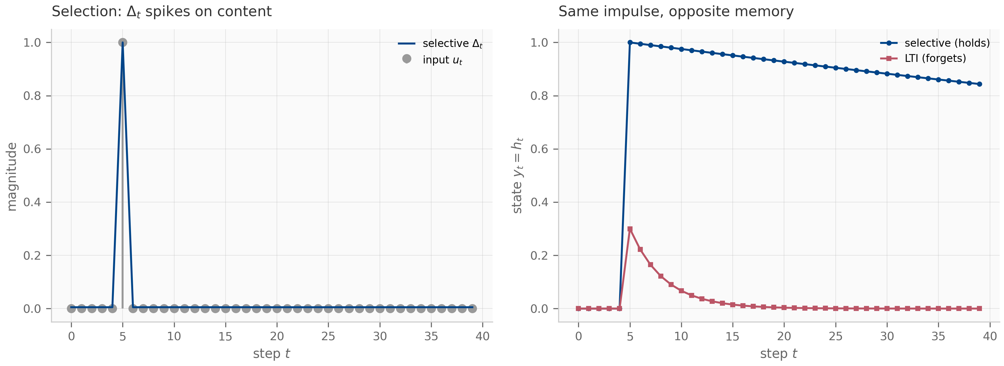
9.3 The selective scan: the §8.6 primitive, now the only route
The convolution is gone (Proposition, §9.1), so the FFT path of training-time S4 has no analogue here. What does survive is the parallel scan of §8.6 — and it survives because it never needed time-invariance in the first place. Recall the associative operator on pairs,
which composes “apply the first affine update, then the second.” Chapter 8 fed it the same at every step; nothing in the operator required that. Feeding it the time-varying pairs scans the selective recurrence directly. This is the selective scan.
(Selective scan equivalence.) The operator is associative for arbitrary first components (not necessarily equal). Its inclusive prefix scan over has as its second components exactly the LTV states , computed in parallel depth Blelloch (1990) . Because no convolution exists (Proposition, §9.1), the FFT path of training-time S4 is gone; this scan recovers depth at linear work and is the primitive the layer is computed with. (Section 9.5 derives a second parallel route — a quadratic matrix multiply — from the same structure.)
The proof (Exercise 9.5, §9.9) is the §8.6 argument with one observation added: the associativity computation never used , so the LTI assumption was load-bearing only for the convolution, never for the scan. The companion pins the equivalence to machine precision — the selective associative scan and the sequential recurrence agree to a measured residual across sequence lengths, which test_selective_scan_equals_sequential holds below .
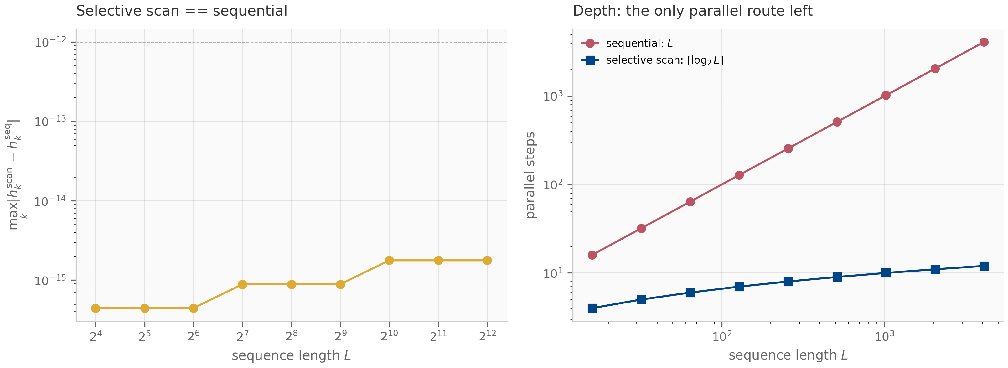
9.4 The hardware-aware fused kernel
Making the scan the only route raises the stakes on computing it efficiently, and the obstacle is memory, not arithmetic. The selective scan’s state is per channel: for a batch of sequences of length with channels and state size , materializing every intermediate state — which the naive backward pass needs — costs , an blow-up over the inputs and outputs. At , , , that is 1.1 GB of fp32 state against 0.067 GB of output (figure below) — at Mamba’s working dimensions, the difference between fitting in memory and not.
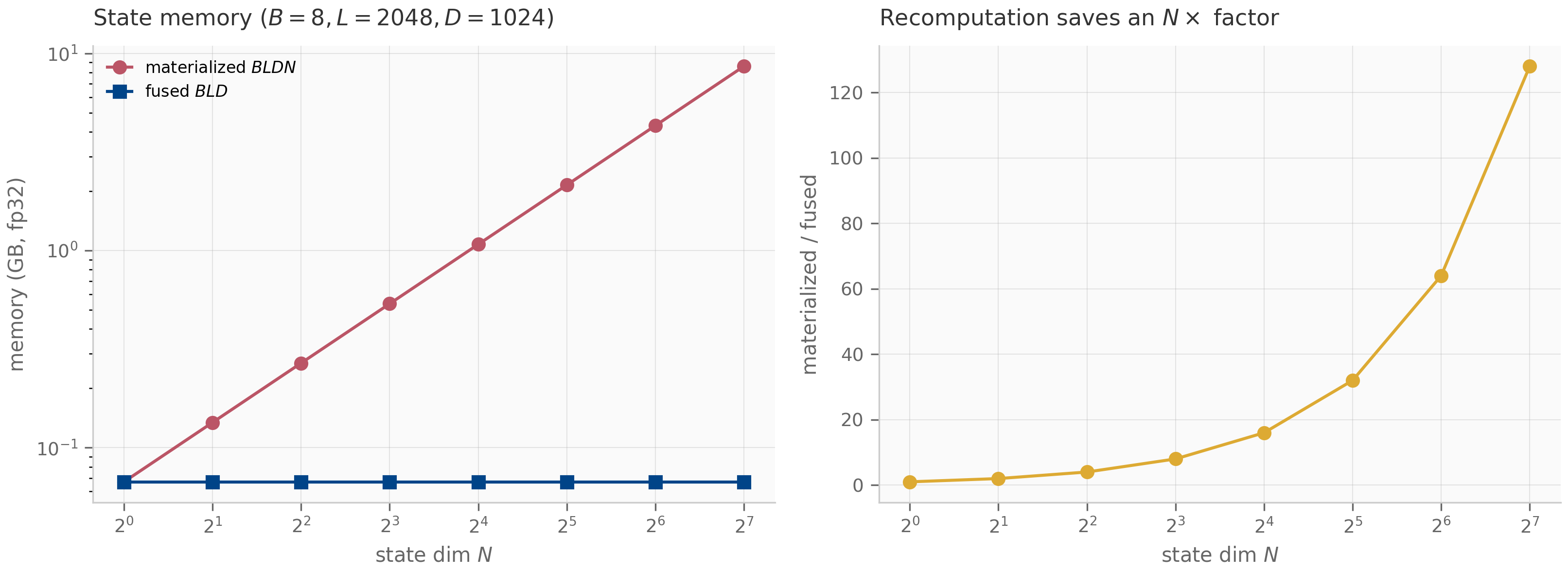
Mamba’s selective-scan kernel resolves this with three hardware-aware moves Gu & Dao (2024)
. It fuses discretization, scan, and output projection into a single GPU kernel, so the expanded state is formed and consumed in fast on-chip SRAM and never written to slow HBM. It recomputes that state in the backward pass instead of storing it — the activation-recomputation trade that pays compute to save memory, the same jax.checkpoint discipline the Mamba-1 reference implementation applies to its selective-scan body. And it exploits the fact, from §9.3, that there is no convolution to fall back on: the scan must be fast, so the engineering goes into the scan rather than into an alternative path. The companion does not implement a CUDA kernel — it makes the memory accounting concrete (the figure above), which is the part that explains why the kernel exists.
9.5 Mamba-2 and SSD: the semiseparable-matrix view
Section 9.2 wrote the inputoutput map entry by entry. Collect those entries into a matrix and a second, matmul-friendly computation appears. Stacking with
and for , gives a lower-triangular matrix. This is the object Mamba-2 organizes the layer around, and it has exactly the structure that makes both computations cheap.
(Structured state-space duality.) For a diagonal state matrix , the selective-SSM output map is -semiseparable: every submatrix lying strictly below the diagonal has rank at most . Consequently admits two computations of the same result — a linear one, the recurrent scan of §9.3 in work and memory, and a quadratic one, forming and multiplying, in work using dense matrix multiplies.
The rank bound is the duality’s engine (Exercise 9.6, §9.9): writing the accumulated decay as with factors each strictly-lower block into a sum of rank-one outer products. The two computations trade off by regime: the recurrent (scan) mode wins for long sequences and autoregressive inference; the quadratic (matmul) mode wins for short chunks, because dense matrix multiplies are what tensor cores do fastest. Mamba-2’s production algorithm chunks the sequence and uses the quadratic mode within chunks and the linear mode across them — both unlocked by the same structure. The companion confirms the two modes agree to a measured residual (pinned below by test_recurrent_equals_matmul) and certifies the rank bound numerically.
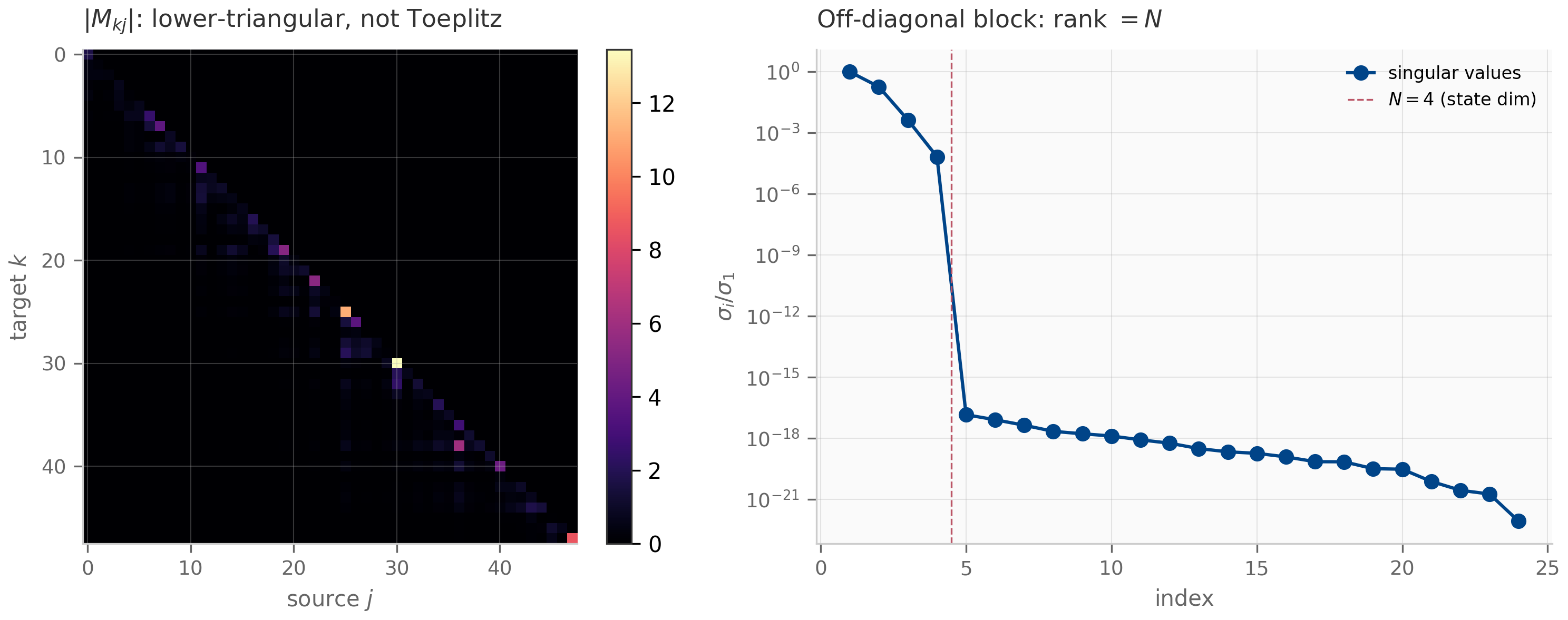
9.6 Duality with linear attention
The semiseparable view pays its largest dividend when the state matrix is a scalar. Mamba-2 restricts — one shared decay per head — which makes the accumulated decay a scalar, , and factors the matrix entry into a decay times an inner product:
with the Hadamard product. Read the right-hand side as attention: are queries, are keys, is the score matrix, are values, and is a causal decay mask in place of softmax. Two things separate it from softmax attention. The mask is fixed by the accumulated step sizes between the two positions, not by a content–content interaction of and ; and the scores enter linearly — there is no softmax nonlinearity — which is precisely what lets the same operator also run in the linear-cost recurrent mode (§9.5). It is linear attention, not softmax attention.
(Selective SSM as masked linear attention.) For scalar , the selective SSM output equals , a masked linear attention with decay mask . The mask is 1-semiseparable (rank-one strictly-lower blocks). The recurrent scan and this masked matmul are the SSM and attention faces of one operator.
This is the formal sense in which “transformers are SSMs” Dao & Gu (2024)
: the linear-attention layer of Katharopoulos et al. Katharopoulos et al. (2020)
and the selective scan compute the same family of contractions, distinguished only by which mode — recurrent or quadratic — is run. The companion verifies the identity as a matrix equation, with the directly-built and the masked-attention form agreeing to (pinned below by test_scalar_A_equals_masked_attention), and certifies that is 1-semiseparable. Chapter 11 enters this same duality from the attention side — linear attention and the delta-rule lineage are the “transformer” reading of the structure this section reached from the SSM side.
9.7 What’s next
The thread of this chapter is one structural change and its consequences. Making depend on the input turns the LTI SSM into a linear time-varying system (§9.2); time-variance breaks the convolution–recurrence duality, so no single kernel exists (§9.1) and the §8.6 associative scan — fed input-dependent transitions — becomes the parallel primitive the layer is computed with (§9.3), which is why Mamba needs a fused, recompute-in-backward kernel (§9.4). Re-reading that scan as a matrix exposes its -semiseparable structure and the recurrent/quadratic duality (§9.5), and for scalar state that matrix is masked linear attention (§9.6).
Chapter 10 keeps selectivity and changes the discretization: Mamba-3 moves to a complex state and replaces zero-order hold with the exponential-trapezoidal scheme of Chapter 4 when the selective dynamics turn stiff Lahoti et al. (2026) . That chapter is where the symplectic-integrator pilot finds its empirical anchor — the selective layer built here, run with a second-order geometric integrator. Chapter 11 takes the §9.6 duality the other way, developing linear attention and the delta-rule lineage as the attention-side reading of the same structured contractions. The selective scan and the semiseparable matrix are the two objects everything downstream reuses.
9.8 Exercises
Six problems mixing computation and theory. Short/numerical (9.1–9.3) have inline collapsible solutions; the theory exercises (9.4–9.6) have full worked solutions in §9.9.
Exercise 9.1 (computation)
Take one stable mode with , and two step sizes: a “write” step and a “hold” step . (a) Compute the discrete transitions and . (b) A value written into the state then held for steps is multiplied by ; compute the retained fraction. (c) Contrast with an LTI system that must use for all steps. What does this say about selectivity?
Solution
(a) (gate nearly open: most of the old state is overwritten), (gate nearly closed: the state is held). (b) Holding for 20 steps retains , about . (c) The LTI system stuck at retains — total forgetting. Selectivity is precisely the freedom to make near on tokens worth holding and near on tokens worth overwriting; a fixed cannot do both, which is the §9.2 figure in two numbers.
Exercise 9.2 (code)
Run companions/ch09/jax/selective_scan_demo.py and confirm the selective associative scan matches the sequential recurrence (the companion reports a residual ). Then explain why the S4 trick of computing the same output by an FFT convolution is unavailable here, referencing Proposition (§9.1).
Solution
The associative scan and the sequential recurrence compute the identical linear recurrence by different reduction orders, so for the same they agree to floating-point error (the companion measures , pinned below ). The FFT path is unavailable because it computes a convolution , which requires a single kernel . By Proposition (§9.1) no such kernel exists once is input-dependent: the map is not Toeplitz, so it is not a convolution, so there is nothing to transform. The scan, by contrast, only needs the per-step pairs and an associative operator, neither of which assumes time-invariance (§9.3).
Exercise 9.3 (computation)
Consider a scalar-state () selective system of length with shared decay , step sizes , scalar projections . Write the entry of the SSD matrix for , and argue that any strictly-lower block (e.g. rows , columns ) has rank .
Solution
With , for . Write , so the accumulated decay is . Then for ,
The block on rows , columns is , an outer product of two vectors — rank . Every strictly-lower block factors the same way, so the matrix is -semiseparable.
Exercise 9.4 (theory) — solution in §9.9
Prove Proposition (§9.1): if the discrete transition is input-dependent, the causal linear map is not Toeplitz, so no convolution kernel with exists. (Hint: a causal linear map is a convolution iff its matrix has constant diagonals.)
Exercise 9.5 (theory) — solution in §9.9
Prove Proposition (§9.3): the operator is associative for arbitrary , and its inclusive prefix scan over reproduces the LTV states . Identify the single place the §8.6 argument used time-invariance and confirm the selective scan does not need it.
Exercise 9.6 (theory) — solution in §9.9
Prove Theorem (§9.5): for diagonal , every strictly-lower-triangular block of the SSD matrix has rank . Then specialize to scalar to derive the masked-attention form of Theorem (§9.6) and show is -semiseparable.
9.9 Full solutions to theory exercises
Solution to Exercise 9.4
A causal linear map on sequences of length is represented by a lower-triangular matrix with . It is a convolution — i.e. — if and only if depends only on the offset , which is exactly the statement that is Toeplitz (constant along each diagonal ).
For the selective system, the diagonal- entry is
Consider the main diagonal (offset ): the accumulated sum is empty, so . Because are input-dependent, varies with whenever the input does, so the main diagonal is not constant and is not Toeplitz. (More strongly, for the factor is not a function of once varies, so no off-diagonal is constant either.) A non-Toeplitz causal map is not a convolution, so no kernel exists; the time-invariant case, where makes depend only on , is the sole case that is Toeplitz.
Solution to Exercise 9.5
Associativity. Write a pair as the affine map (with acting elementwise). Composition of affine maps is associative because function composition is; concretely, with as defined,
and the two agree. Nowhere did this computation assume — that is the single place §8.6 silently used (and did not need) time-invariance. Prefix scan. Let and let be the inclusive scan. By induction on the second component of equals : for it is (from ); and has second component . Since is associative, all prefixes are computable by a balanced reduction tree in depth Blelloch (1990) . The selective scan is thus the §8.6 scan verbatim, with time-varying in place of a constant — the operator’s associativity never cared.
Solution to Exercise 9.6
Semiseparability. Fix a strictly-lower block: rows and columns with , so throughout and the accumulated sum is nonempty. Write , so and . Then
with and . As a matrix the block is with , , hence rank . Every strictly-lower block has this form, so is -semiseparable. (The factorization is exactly what the chunked algorithm exploits: is read out from the per-chunk states, folded into them.)
Scalar specialization. Put , i.e. for all . The decay no longer depends on , so it pulls out of the sum:
with . In matrix form , the masked-attention form of Theorem (§9.6): is the score matrix and the decay mask. Finally for , so any strictly-lower block of is the outer product — rank one. Thus is -semiseparable, and the full is -semiseparable with the state size (here the rank of the score matrix).
9.10 Companion code
Two language tracks for Chapter 9 — JAX (the reference, with the parallel selective scan and the semiseparable-matrix tools) and PyTorch (the nn.Module layers and the masked-attention dual). Julia is omitted, as in Chapter 8: the selective scan and the SSD matrix are the same algorithm in any language, and the JAX/PyTorch pair already carries the cross-framework lesson. The two tracks are pinned bit-for-bit against each other in float64.
JAX (companions/ch09/jax/):
selective_ssm.py— the SISO selective-SSM core: the selection mechanism, the per-step ZOH discretization, and the selective scan viajax.lax.associative_scanwith its sequential oracle. The §9.3 equivalence lives here.selective_vs_lti.py— emitsselective-vs-lti.png(§9.2): the held-vs-forgotten single-mode contrast.selective_scan_demo.py— emitsselective-scan.png(§9.3) andmemory-cost.png(§9.4): scan-vs-sequential agreement and depth, and the materialized-vs-fused memory accounting.ssd_semiseparable.py— the SSD tools:segsum, the semiseparable matrixbuild_ssm_matrix, the rank certificateis_n_semiseparable, and the scalar-masked_attention_form; emitssemiseparable.png(§9.5).tests/—test_selective.pypins the selective scan-equivalence, stability by construction, and the not-Toeplitz collapse;test_ssd.pypins the recurrent-vs-matmul duality, -semiseparability, and the scalar- masked-attention identity.
PyTorch (companions/ch09/torch/):
selective_ssm.py— the selective SSM as annn.Module(A_loga learnablenn.Parameter, selection projections asnn.Linear, eager sequential scan), plus the functional core mirrored from JAX.ssd_matmul.py— the scalar- dual form asSSDAttention: masked linear attention with the decay mask in place of softmax.tests/test_selective_torch.py— cross-framework parity: the torch selective scan and SSD matrices equal their JAX counterparts to within .
To run from the repo root:
# JAX (uses the uv .venv with jax, numpy, matplotlib)
PYTHONPATH=. python companions/ch09/jax/selective_vs_lti.py
PYTHONPATH=. python companions/ch09/jax/selective_scan_demo.py
PYTHONPATH=. python companions/ch09/jax/ssd_semiseparable.py
# PyTorch (needs the .venv [torch] extra)
PYTHONPATH=. python companions/ch09/torch/selective_ssm.py
PYTHONPATH=. python companions/ch09/torch/ssd_matmul.pyAll figures emit to public/figures/ch09/.
Mamba-3 and the exponential-trapezoidal integrator
How Mamba-3 keeps selectivity and changes two things — a second-order exponential-trapezoidal integrator and a complex state — turning the dynamical-systems lens of Chapters 4-6 onto a production sequence model.
Mamba-3 and the exponential-trapezoidal integrator
10.1 Two upgrades to the selective SSM
Chapter 9 built the selective SSM: input-dependent make the dynamics linear time-varying, the convolution view collapses, and the selective scan plus the semiseparable-matrix view (SSD) carry the computation. Mamba-1 and Mamba-2 both discretize with zero-order hold (ZOH) and keep a real diagonal state matrix .
Mamba-3 Lahoti et al. (2026) changes two things of dynamical-systems substance and leaves the rest of the SSD scaffold (the semiseparable structure of Theorem 9.4, the scan, the attention duality of Theorem 9.5) intact:
- A second-order integrator. ZOH is first-order accurate; Mamba-3 adopts a second-order exponential-trapezoidal scheme — the exponential-integrator idea of Chapter 4 §4.5 in its trapezoidal-quadrature form (§10.2) — while keeping ZOH’s exact treatment of the homogeneous dynamics (§10.2-10.3).
- A complex state. A real diagonal mode can only decay; a complex mode decays and rotates, so a single head becomes a damped oscillator (§10.4).
Both changes are dynamical-systems moves, and both have been waiting since the foundations chapters: the integrator is the Chapter 4-5 story applied to a real architecture, and the complex state is the spiral phase portrait of Chapters 1-2. The C1 pilot’s empirical question — whether a second-order, structure-preserving integrator actually buys accuracy on a selective SSM without costing stability — is the through-line.
10.2 The exponential-trapezoidal scheme
Recall the continuous mode , whose exact one-step map is . Every exponential integrator keeps the transition exact (the philosophy of Chapter 4 §4.5) and approximates only the forcing integral. ZOH holds the input constant at the left endpoint; the exponential-trapezoidal scheme applies the trapezoidal quadrature rule to the forcing integral — averaging the integrand at the two endpoints. The integrand is at and at , so the rule gives . Weighting the two endpoints by gives the three-term update
The contrast with ZOH is the third term: where ZOH reads only the left endpoint , the trapezoid reads both endpoints. At this is the symmetric trapezoidal rule (globally second-order); at it collapses to a shifted ZOH (first order). Mamba-3 makes itself input-dependent (a sigmoid of a learned projection), one more selective knob.
This single fact — that is identical for the two schemes — has a sharp consequence for how the order can be measured.
For the exponential-trapezoidal scheme has local truncation error per step, hence global order 2, provided the input is non-constant and . On the homogeneous system () both ZOH and exp-trapezoidal reproduce the exact solution to machine precision, so the order difference is unobservable there.
The proof is Exercise 10.4 (§10.9). The practical reading is a trap worth naming: because the homogeneous transition is exact, a convergence study run on an autonomous system shows ZOH and exp-trapezoidal as identical lines at roundoff — the second order is simply not visible. The companion confirms this directly: on the autonomous mode both schemes sit at , while on the forced mode the fitted convergence slopes separate cleanly into (ZOH) and (exp-trapezoidal). This is the same lesson Chapter 4 flagged in Exercise 4.3 (“setting makes ZOH exact; the slope is meaningless”), now load-bearing for verifying a real architecture’s headline claim.
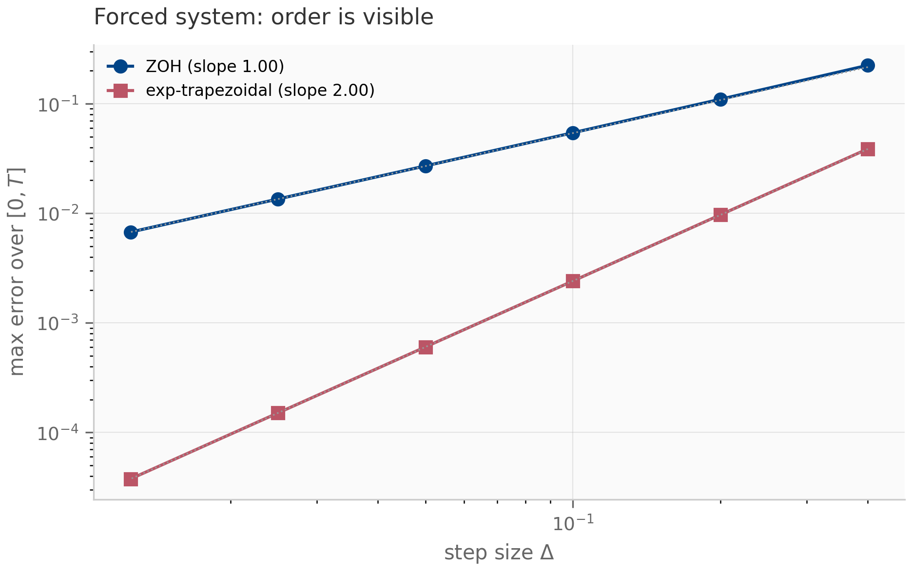
10.3 Stability and accuracy decouple
Why adopt an exponential integrator rather than a higher-order Runge-Kutta method? Because the exponential transition is exact, the discrete amplification factor is , which is for any stable mode () at any step size. ZOH and exp-trapezoidal are therefore unconditionally stable on the homogeneous part — A-stable over the entire left half-plane — and, crucially, stability is set by alone, independent of the order of the forcing quadrature. For a Runge-Kutta method a single stability polynomial controls both accuracy and the stability region; the exponential integrator decouples them.
For , the exponential-trapezoidal (and ZOH) amplification factor satisfies for every , and as the mode stiffens (). The bilinear (Tustin) scheme is also A-stable but uses the -Padé approximation , for which as the mode stiffens: stiff modes are left undamped.
The proof is Exercise 10.6 (§10.9). The companion makes the contrast quantitative: at a stiff , the exponential schemes give (fully damped) while bilinear gives (still ringing). This is why an exponential integrator is the right tool when the input-dependent of a selective SSM produces stiff dynamics, as Chapter 4 §4.5 anticipated for exactly this chapter. One caveat matters for §10.4: the theorem bounds the magnitude only. For a complex mode it says nothing about how faithfully the discrete rotation tracks the continuous phase — phase fidelity is a separate question, and the open one the frontier paragraph below raises.
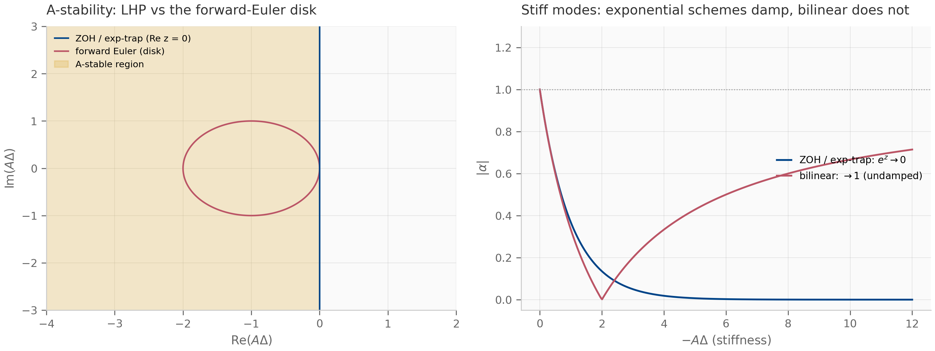
The geometric-integrator frontier (where the pilot goes next). Exp-trapezoidal is a second-order exponential integrator; it is not symplectic. For the oscillatory complex modes introduced in §10.4, the question the symplectic-integrator pilot asks is whether a geometric integrator (Chapter 6) — one that preserves a phase-space invariant rather than merely a damping bound — controls long-horizon phase error better than exp-trapezoidal does. That is an open empirical question, not a settled result, and it is the heart of the “discretization stability atlas” the pilot pursues; Chapter 17 returns to it. This chapter establishes the settled part: exp-trapezoidal is second-order, A-stable, and exact on the homogeneous part.
10.4 Complex state: decay and oscillation in one head
A real diagonal mode gives : pure geometric decay, a single forgetting timescale. Mamba-3 lets the mode be complex, , so
The magnitude decays at rate per unit step and the phase advances by : a single head is now a damped oscillator, tracing the logarithmic spiral of Chapters 1-2 rather than a monotone decay. This lets one head represent an oscillatory feature — a frequency — instead of only a timescale.
In production Mamba-3 never stores a complex dtype. It keeps a real state and applies rotary position embeddings (RoPE) — 2-D rotations — to the projections . The justification is the elementary isomorphism between complex multiplication and rotation-scaling.
Representing as the real vector , multiplication by equals applying the scaled rotation . Consequently the complex recurrence and the real 2-D recurrence produce identical trajectories.
The proof is Exercise 10.5 (§10.9). The companion pins the two recurrences equal to under a random complex drive, and confirms the spiral’s decay rate equals exactly — the empirical content of “decay and oscillation in one head.”
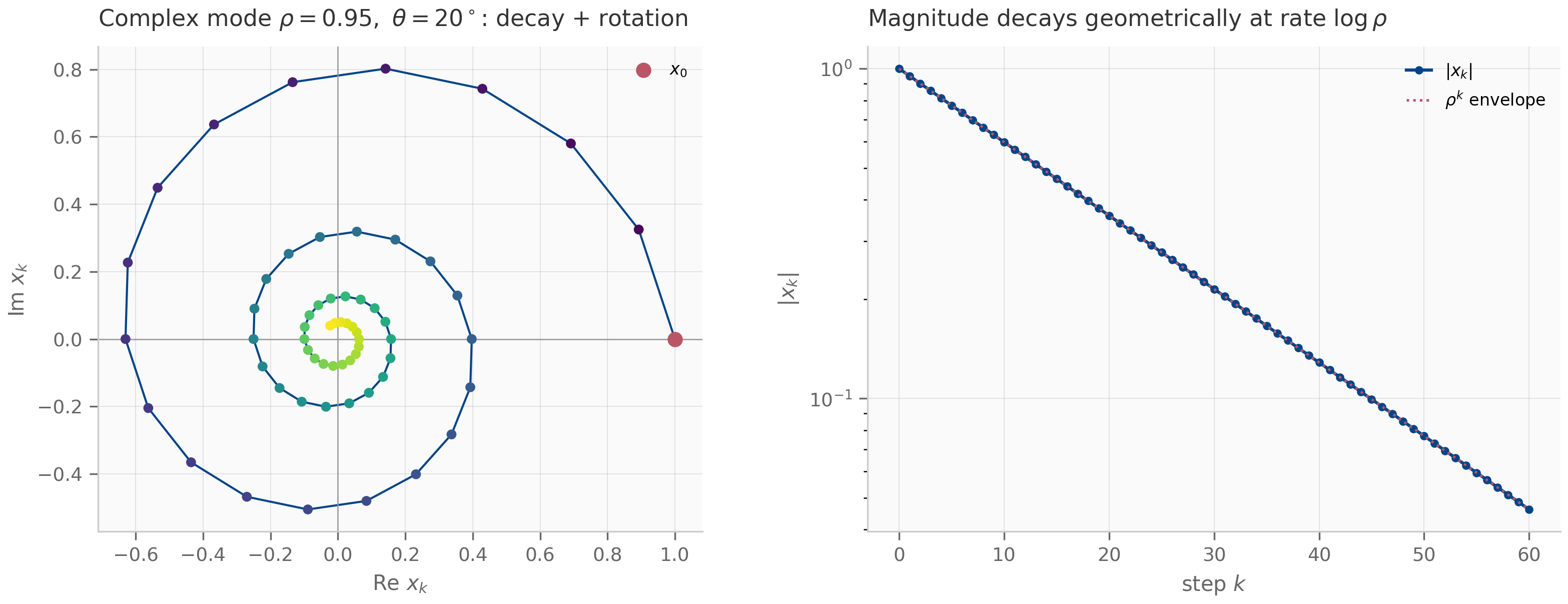
10.5 The trapezoidal SSD pass
The second-order stencil must coexist with the SSD machinery of Chapter 9 — the semiseparable matrix that lets the layer run as a parallel matmul or a linear-time scan. It does, because only the injection stencil changes. Unrolling the trapezoidal recurrence with the state-transition operator (the same as Definition 9.2) splits the output into two semiseparable streams that share the one decay : a right-endpoint stream weighting source by , and a left-endpoint stream weighting source by across the strictly-lower triangle. Both reuse the Chapter 9 segment-sum decay; the order-2 upgrade is two cheap masked matmuls in place of one.
The companion verifies that the dense two-stream matmul reproduces the sequential trapezoidal recurrence to (for both real and complex modes), and that the end-to-end output is genuinely second-order — halving the step size cuts the error by a factor of four. The SSD duality of §9.5 survives the integrator upgrade intact: same matrix, two schedules, now order 2.
10.6 MIMO and the production block
Two further Mamba-3 changes sit outside the integrator-and-state story this chapter develops, and we treat them briefly. MIMO rank- state mixing (the input and output projections each gain a rank- dimension) raises decode-time arithmetic intensity at fixed state size and, Mamba-3 reports, also lifts model quality through the added expressivity (a -point average downstream gain over the SISO variant) — but neither effect changes the discretization or stability story. The full production block — SwiGLU gating, QK-normalization, the bias — wraps the layer studied here; those too are orthogonal to the integrator-and-state question, and we point to the reference implementation rather than reproduce them Lahoti et al. (2026) .
What this chapter isolates is the dynamical-systems substance: a selective SSM (Chapter 9) run with a second-order exponential integrator (Chapters 4-5) and a complex state (Chapters 1-2, 8). The open program — whether geometric integrators (Chapter 6) preserve long-horizon phase structure better than the exponential scheme over the learned eigenvalue spectrum — is the discretization stability atlas the C1 pilot builds, and Chapter 17 returns to it.
10.7 What’s next
Mamba-3 kept Chapter 9’s selectivity and changed two things: a second-order exponential-trapezoidal integrator (accuracy in the forcing, stability from the exact exponential) and a complex state (decay and oscillation in one head), realized via RoPE and computed through the trapezoidal SSD pass. This closes the core SSM line — HiPPO (Chapter 7) to LTI S4/S4D/S5 (Chapter 8) to selective Mamba (Chapter 9) to Mamba-3 (here).
Chapter 11 opens the “beyond SSM” part by taking the SSD duality of §9.6 the other way: linear attention and the Hyena long-convolution lineage enter from the attention side of Theorem 9.5, where the structured contractions of these four chapters reappear wearing transformer clothing.
10.8 Exercises
Six problems: three short (inline solutions), three longer (full solutions in §10.9).
Exercise 10.1 (short)
For a complex mode with , , and step , compute and the phase advance of over two steps. Which is the decay timescale and which is the oscillation frequency?
Solution
, so per step and the phase advances per step. Over two steps and the phase advances . The magnitude sets the decay timescale; sets the oscillation frequency. They are independent — that is the point of a complex mode.
Exercise 10.2 (short, code)
Run companions/ch10/jax/discretization.py. Confirm the fitted convergence slopes
are for ZOH and for exp-trapezoidal on the forced system.
Then explain, in one sentence, why the same script reports both schemes at
on the homogeneous system.
Solution
The script prints ZOH slope and exp-trapezoidal slope on the forced mode. On the homogeneous mode the transition is exact for both schemes, so both reproduce to floating-point roundoff and the order difference — which lives entirely in the forcing coefficients — never enters (Theorem 10.1).
Exercise 10.3 (short)
Write the exp-trapezoidal coefficients for , , and . Show that reduces to a first-order shifted ZOH (no current-input term carrying the decay).
Solution
throughout. : , (pure left endpoint). : , (symmetric). : , — only the current input enters, with no decay applied to it, which is a first-order ZOH shifted by one step. The symmetric is the only second-order member.
Exercise 10.4 (theory) — solution in §10.9
Prove Theorem 10.1: for the exponential-trapezoidal scheme has local truncation error on a forced system, and show that on the homogeneous system both ZOH and exp-trapezoidal are exact.
Exercise 10.5 (theory) — solution in §10.9
Prove Theorem 10.3: that a 2-D rotation by on equals multiplication of by , and conclude the complex and real-RoPE recurrences coincide.
Exercise 10.6 (theory) — solution in §10.9
Prove Theorem 10.2: that the exponential schemes are A-stable with on stiff modes, and contrast the bilinear Padé factor, showing as .
10.9 Full solutions to theory exercises
Solution to Exercise 10.4
Write the exact one-step map by variation of constants over :
The transition is reproduced exactly by both schemes, so all error is in the forcing integral. Exp-trapezoidal approximates , with integrand , by the trapezoidal quadrature rule — the endpoint weights of §10.2. The trapezoidal rule on an interval of width has error for some interior ; since is whenever is , the local truncation error is per step, and summing steps over a fixed horizon yields global order 2. For the homogeneous system the forcing integral vanishes identically and exactly for both schemes, regardless of order — there is no forcing term to approximate, so the order distinction disappears.
Solution to Exercise 10.5
Let and write . Then
whose real-vector form is with . Scaling by commutes with the real isomorphism, so multiplication by is on . Applying this at every step of the affine recurrence (the additive drive maps to componentwise, which the isomorphism also preserves) shows the complex recurrence and the real recurrence produce identical trajectories under .
Solution to Exercise 10.6
For the exponential schemes , so . If and then the exponent is negative and for every (A-stability over the whole left half-plane), and as the mode stiffens () we have . For the bilinear scheme with ; writing with , (the left point is closer to , the right to ), so — also A-stable. But as the ratio , so : stiff modes are mapped to the unit circle and ring rather than decaying. This is the qualitative gap the exponential transition closes.
10.10 Companion code
The companions live in companions/ch10/{jax,julia,torch}/. The JAX module covers
the integrator, the complex state, and the trapezoidal SSD pass; the PyTorch module
mirrors the integrator and complex state (cross-framework parity); the Julia module
is the discretization atlas only — the numerical-analysis core — and joins the
Chapter 4-6 Julia family that the C1 pilot’s stability atlas builds on.
The discretization study (order slopes, homogeneous-blindness, stability regions):
PYTHONPATH=. python companions/ch10/jax/discretization.py
julia --project=companions/ch10/julia companions/ch10/julia/discretization.jlThe complex state and RoPE equivalence (the spiral figure):
PYTHONPATH=. python companions/ch10/jax/complex_state.pyThe trapezoidal SSD pass (matmul equals the sequential oracle):
PYTHONPATH=. python companions/ch10/jax/trapezoidal_ssd.pyThe PyTorch mirror (integrator and complex state, parity-checked against JAX):
PYTHONPATH=. python companions/ch10/torch/discretization.py
PYTHONPATH=. python companions/ch10/torch/complex_state.pyRun the suites — JAX and Julia in the fast loop, torch separately:
make companion-jax-tests
make companion-julia-tests
make companion-torch-testsLinear attention and Hyena: long convolution and gated recurrence
Linear attention read as a matrix-state linear recurrence — the dual of Chapter 9's scan, entered from the attention side — then gated into the LTV/selectivity face (GLA, RetNet), pivoted to Hyena's implicit LTI long convolution, and landed honestly on the associative-recall capacity limit of any finite state.
Linear attention and Hyena: long convolution and gated recurrence
11.1 From softmax to separable scores
Chapter 9 reached a striking identity from the state-space side: a scalar-state selective SSM is masked linear attention (Theorem 9.5). The scan’s path-ordered taps reassemble into a single lower-triangular matrix , with a causal decay mask replacing the softmax. This chapter enters that same duality from the other side. We start with attention and rediscover the state space.
Causal attention computes, for each position ,
The exponential couples every query to every key: the normalizer cannot be factored across , so the only way to evaluate it is to materialize all scores. The move that breaks the coupling Katharopoulos et al. (2020) is to choose a feature map with non-negative entries and write the similarity as an inner product of features,
Separability is the whole engine. Because factors, the numerator and denominator each become a query contracted against a running sum over keys — and a running sum is a state.
11.2 Linear attention as a matrix-state recurrence
Fix . Define a matrix state and a normalizer by
with , . This is a bona fide state-space recurrence: the hidden state is a matrix, the transition is the identity (, pure accumulation with no forgetting — the LTI face of Chapter 8), and the input is injected as the rank-one outer product . It is Chapter 9’s scan with the carry promoted from a vector to a matrix and the decay switched off.
The same operator has a second, parallel face. Stacking and , the unnormalized output is a masked matrix product.
For any feature map , the recurrent form (, output ) and the parallel form
with the all-ones causal mask, compute the identical output. The recurrent form costs time and memory; the parallel form costs . This is exactly Theorem 9.5 with the decay mask specialized to ones.
The proof (Exercise 11.4, §11.9) is one line of reassociation: , so , which is precisely row of . The mask supplies the causal cumulative sum that the recurrence performs incrementally. The companion confirms the two routes agree to machine precision in float64: at , flat across sequence lengths.
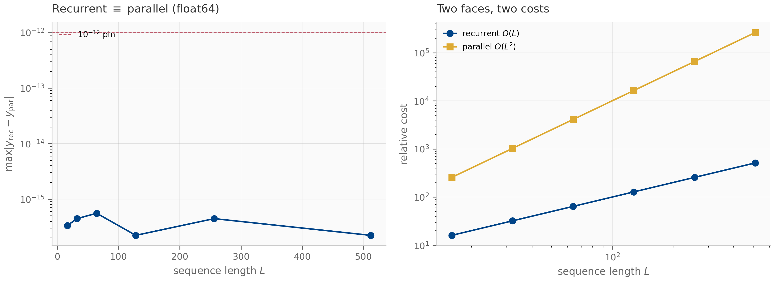
The normalizer, and why this chapter is float64. The denominator is a large-over-large quotient: both and the numerator grow like , so the ratio is a difference of accumulations prone to catastrophic cancellation in low precision. The recurrent and parallel forms accumulate that quotient in different orders (sequential cumsum versus a single matmul), so their agreement is a direct probe of arithmetic precision. In float64 they match to at ; in float32 the same computation caps out at — a precision gap of nearly . The identity pin is simply unreachable in single precision, which is why every companion in this chapter runs float64. (Gated linear attention in §11.3 sidesteps the issue by dropping the normalizer for an explicit decay plus an output normalization — cleaner numerically.)
11.3 Gating: GLA, RetNet, and the LTV reading
Ungated linear attention never forgets. To make it selective — to let the state forget — attach a per-step gate to the transition:
This is the Chapter 9 selectivity move read from the attention side. Two regimes sit inside it:
- RetNet Sun et al. (2023) takes , a fixed head-wise decay. The transition is constant, so the operator is LTI with forgetting — the Chapter 8 face plus a decay. Its parallel decay mask is Toeplitz (it depends only on the lag ).
- GLA Yang et al. (2024) and HGRN2 Qin et al. (2024) make data-dependent. The transition now changes every step, so the operator is LTV — input-dependent forgetting, exactly the selectivity of Chapter 9. Its decay mask is not Toeplitz; the diagonals vary, just as Chapter 9’s selective decay mask does.
The masked-parallel form generalizes by the GLA “secondary” rescaling: with the cumulative log-gate , set and ; then is the gated score. This is what makes the duality exact.
The gated recurrence , , has a masked-parallel form. For a scalar per-step gate it is exactly with the 1-semiseparable decay mask , and under this coincides exactly with the decay mask of Theorem 9.5 — gated linear attention and the scalar-state selective SSM are the same operator, read from opposite sides. For a per-feature gate the decay acts per channel and does not collapse to a single scalar mask; the parallel form instead rescales features by the cumulative gate (, , ), recovering the same recurrence (§11.9).
The proof is Exercise 11.5 (§11.9): unroll the gated recurrence, contract with
, and recognize the product-of-gates as the cumulative decay that
Theorem 9.4‘s segsum exponentiates. The companion both
checks the recurrent–masked identity ( difference for
a data-dependent gate) and verifies the cross-chapter bridge against the actual
Chapter 9 code: the GLA scalar mask and Chapter 9’s segsum mask agree to
(bit-identical) under .
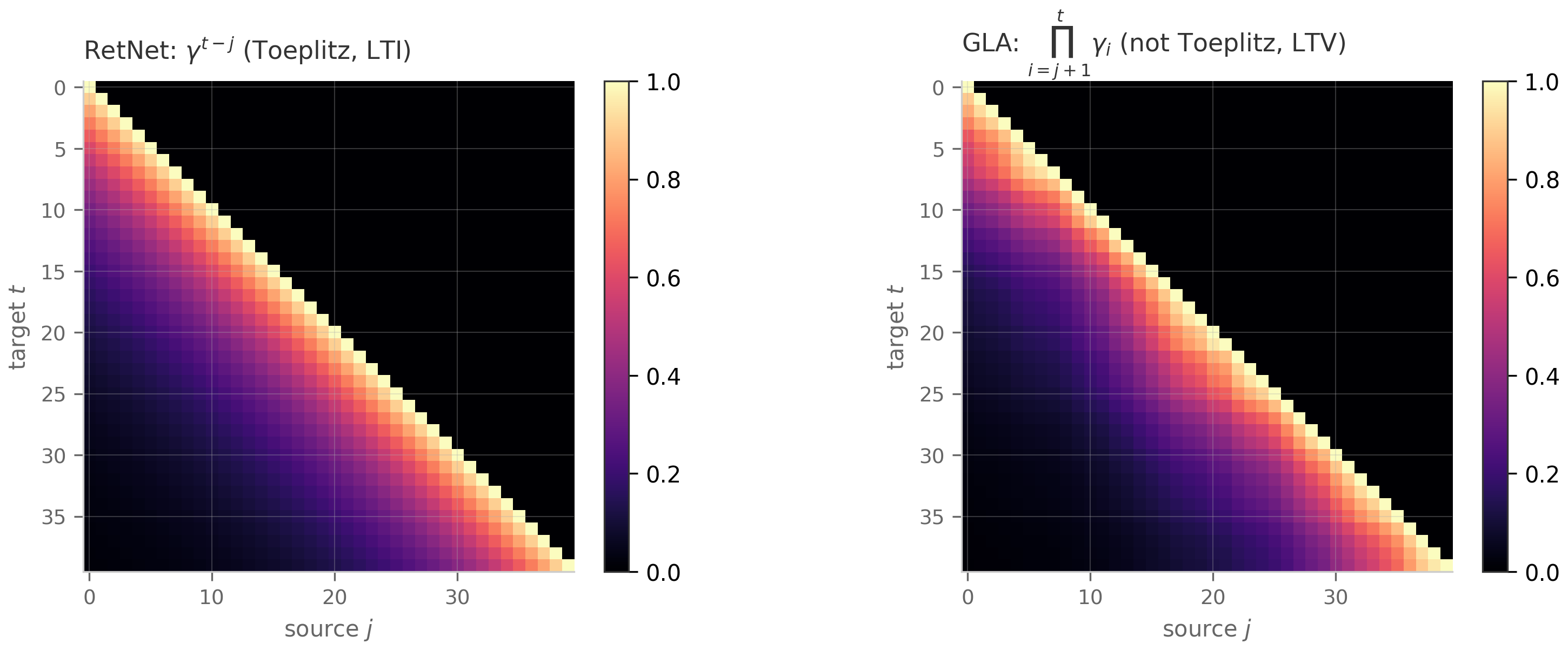
11.4 Hyena: the FFT long convolution
The second operator family of this chapter abandons attention entirely — yet it is the same structural idea in new dress, not a digression: Hyena’s convolution is one more instance of the LTI/LTV fork that organized §§11.2–11.3, as §11.5 will make explicit. Hyena Poli et al. (2023) interleaves implicit long convolutions with elementwise multiplicative gating. The convolution is the object to teach: a causal long convolution is a linear time-invariant operator — the convolutional view of an SSM (Proposition 8.1) — computable in by the FFT rather than the explicit Toeplitz product. For input and a per-channel filter ,
The one subtlety is causality under the cyclic FFT.
Padding and the filter to length , multiplying their real FFTs pointwise, inverse-transforming, and truncating to the first samples yields exactly the lower-triangular Toeplitz product above. Padding to (in fact any ) is sufficient: it sends the cyclic FFT’s wrap-around terms onto the zero-padded tail of , where they contribute nothing. The un-padded length- transform wraps late taps onto early outputs and breaks causality, so some padding past is required.
The proof is Exercise 11.6(a) (§11.9). The companion makes both halves concrete: the FFT route reproduces the explicit-Toeplitz oracle to in float64 (the predecessor implementation ran float32 at a tolerance — this is a tightening), while the un-padded variant disagrees with the oracle by , an violation of causality.
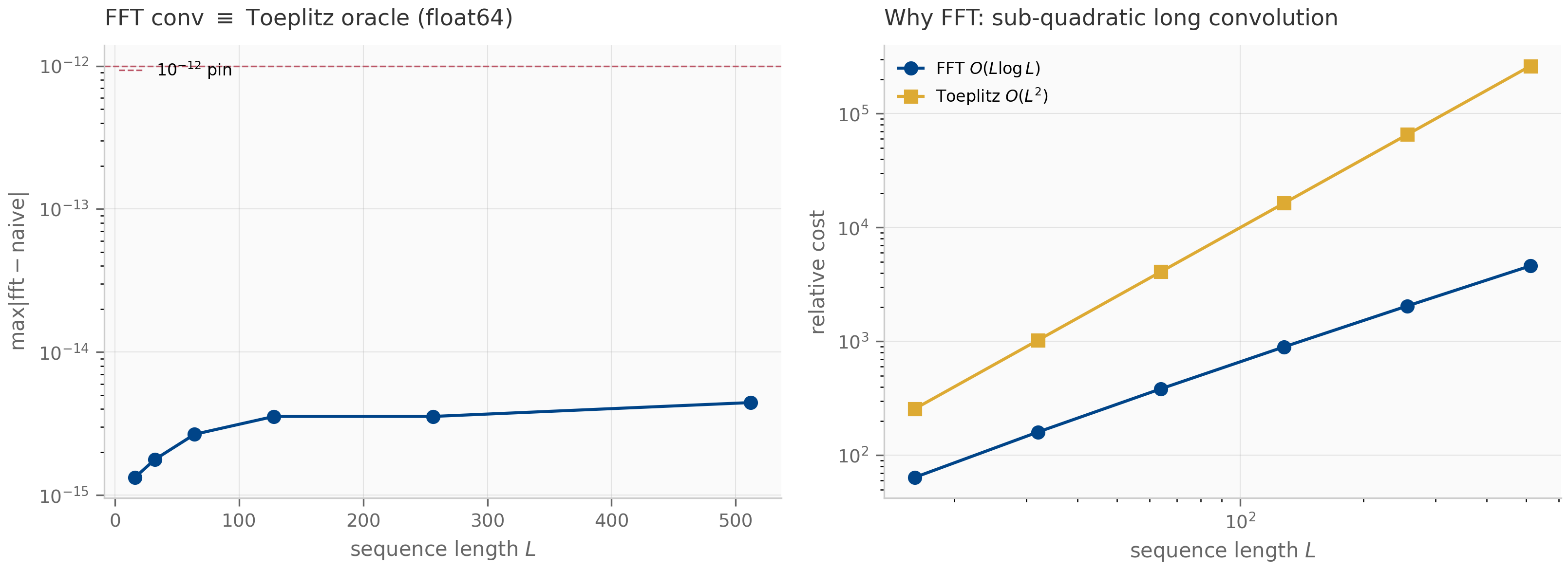
11.5 Implicit and selective filters
What does the long convolution mean in the dynamical-systems vocabulary of this book? Everything hinges on whether the filter is fixed or input-dependent.
When the filter is static across the batch and sequence, is a single linear time-invariant convolution — one kernel, the convolutional face of an SSM (Proposition 8.1). S4 lives exactly here: its kernel is materialized from a structured continuous-time ODE, and the same FFT machinery of §11.4 applies. Hyena keeps the unrestricted kernel and pays the factor, where S4 and Mamba fix the kernel shape — a structured semiseparable matrix (Theorem 9.4) — to buy .
When the filter is made input-dependent — the “selective Hyena” variant, where the convolution kernel itself is a function of the input — time-invariance breaks, exactly as Chapter 9’s input-dependent broke it. No single kernel exists; no convolution theorem applies; the operator rejoins the LTV family of §11.3. This is the same fork seen three times now: a fixed transition is LTI and admits a convolution or a closed-form mask; an input-dependent transition is LTV and admits only the scan. Hyena’s gating, GLA’s decay, and Mamba’s selection are three spellings of one move.
11.6 Counter-evidence: associative recall and capacity
Beyond-SSM does not mean better-than-SSM. The honest place to end is where linear attention loses: multi-query associative recall (MQAR) — store key–value pairs, then answer queries by retrieving the value bound to a key Arora et al. (2024) . On this task, linear attention degrades as grows while selective SSMs (Mamba) and softmax attention stay near-perfect. The mechanism is the §11.2 insight turned into a limitation, and it is provable.
The linear-attention state is a sum of rank-one matrices, so . If , the feature vectors are linearly dependent, so the readout cannot reproduce linearly independent values: there exist queries for which exact recall is impossible, regardless of . Capacity is bounded by the feature dimension.
The proof is Exercise 11.6(b) (§11.9). The companion turns the bound into a measured fact (a fixed-weight mechanism, not a trained model — the trained-model accuracy curves are cited to Zoology Arora et al. (2024) ). Storing random unit keys with orthonormal values and reading each back, the per-binding retrieval error behaves exactly as the rank bound predicts:
- Below capacity, exact. With orthonormal keys the features are independent, the state is full-rank, and recall is exact — error .
- Past capacity, degrading. With generic keys the error grows like : at it is for and for (capacity scales with the state size), rising to at .
- The oracle stays exact. Softmax attention’s exponential sharpening concentrates the readout on the self-match, so its error is independent of — the capacity-unbounded baseline that linear attention cannot match.
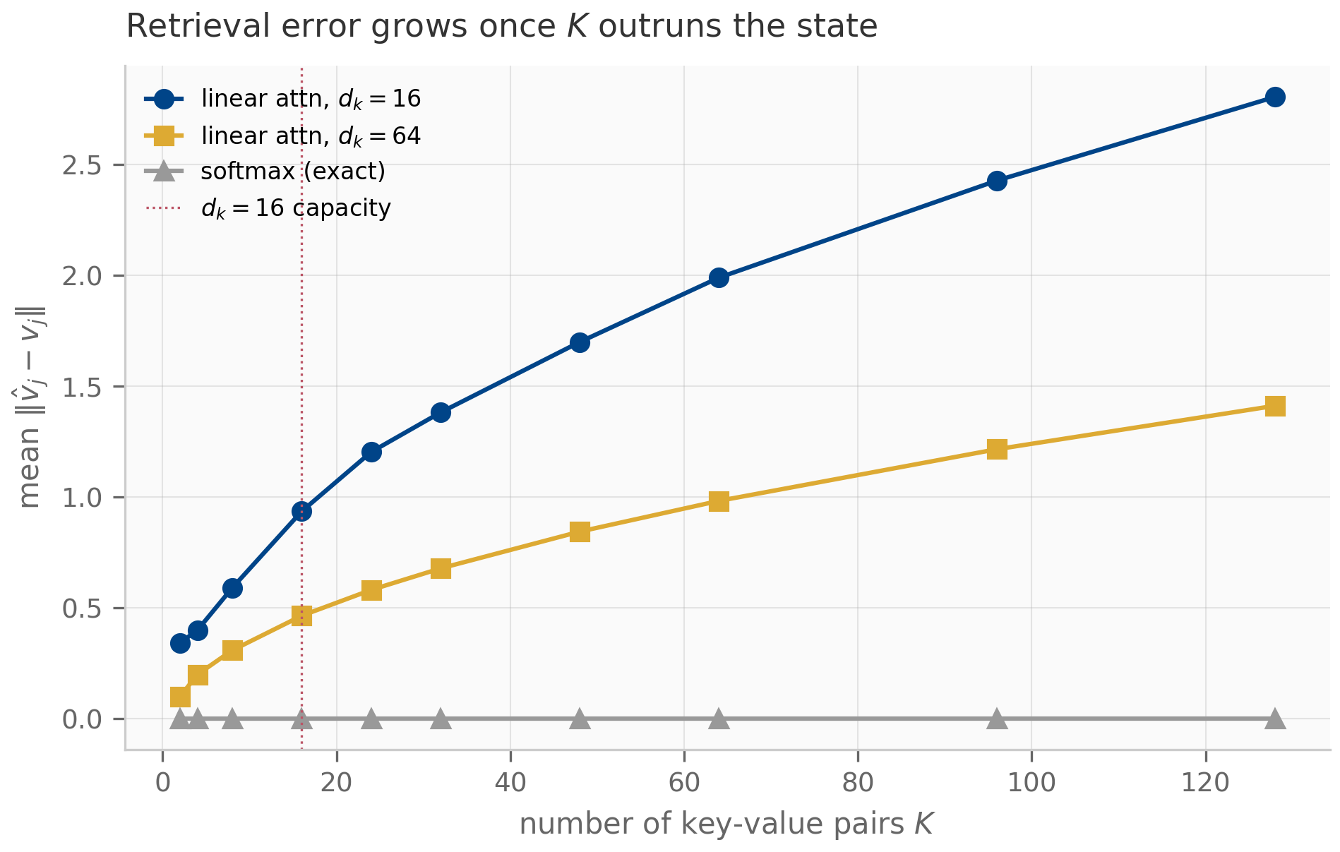
Gating (§11.3) helps at the margin — a decay lets the state shed stale bindings — but it reweights a finite state, it does not raise the rank ceiling. Closing the gap needs either a genuinely larger structured state (the selective-SSM route of Chapters 9–10) or a smarter write rule, which is the subject of Chapter 12.
11.7 What’s next
This chapter built the linear-attention half of the “beyond-SSM” family: an additive matrix-state recurrence (), gated into the LTV/selectivity face (GLA, RetNet), with Hyena’s implicit LTI long convolution as the sibling operator and a hard capacity limit (§11.6) at the bottom.
Chapter 9 promised this chapter would develop “linear attention and the delta-rule lineage” as the attention-side reading of structured contractions. We have built the linear-attention half; the delta-rule half sharpens exactly the §11.6 capacity limit. Instead of blindly accumulating , the delta rule overwrites the value currently associated with a key — a rank-one correction
turning the identity-transition recurrence into a genuinely data-dependent write. That is Chapter 12 (the online-learning reading: DeltaNet as explicit-Euler, Longhorn as backward-Euler). Chapter 13 adds exponential gates and matrix memory (xLSTM, RWKV-7); Chapter 14 mixes these layers with attention into the production hybrids. The structure is one family; we are still mapping its faces.
11.8 Exercises
Three short problems (solutions inline) and three longer ones (solutions in §11.9).
Exercise 11.1 (short)
Take , , and two key–value pairs with scalar values. Write explicitly as a sum of two outer products, and verify by hand that the unnormalized readout for a query equals row of the masked-attention form .
Solution
(a matrix since is scalar). Then . Row of the masked form is with for — identical (taking ). The outer-product sum and the masked row are two evaluations of the same contraction.
Exercise 11.2 (short, code)
Run companions/ch11/jax/linear_attention.py. Confirm the
recurrent and parallel forms agree to , and explain in one sentence
why the mask here is all ones below the diagonal, whereas Chapter 9’s mask
carried a decay.
Solution
The script prints . The mask is all-ones because ungated linear attention has transition : nothing decays between positions, so the weight on key at query is for every . Chapter 9’s mask carried because its transition decays the contribution of older positions. Gating (§11.3) restores that decay.
Exercise 11.3 (short)
Show that a constant gate reduces the GLA decay mask to RetNet’s , and explain in one line why a constant gate makes the mask Toeplitz while an input-dependent does not.
Solution
. This depends only on the lag , so is constant along each diagonal — Toeplitz. With input-dependent the product depends on which steps are spanned, not just how many, so equal-lag entries on a diagonal differ — the mask is no longer Toeplitz. (The companion’s RetNet mask has Toeplitz residual exactly .)
Exercise 11.4 (theory) — solution in §11.9
Prove the recurrent–parallel equivalence of §11.2: the recurrent matrix-state form and the masked-parallel form compute the same output, and state the time/memory cost of each.
Exercise 11.5 (theory) — solution in §11.9
Prove the gated-linear-attention duality of §11.3, and identify the exact correspondence under which the scalar-gate GLA mask coincides with the Chapter 9 decay mask of Theorem 9.5.
Exercise 11.6 (theory) — solution in §11.9
(a) Prove the FFT-causality theorem of §11.4 — that padding past (to ) lets the FFT compute the causal convolution, while the un-padded transform does not. (b) Prove the rank bound of the §11.6 capacity proposition, and connect it to the growth of retrieval error in the §11.6 capacity figure.
11.9 Full solutions to theory exercises
Solution to Exercise 11.4
Unrolling the recurrence from gives . Hence
Row of the parallel form is , since . The two are identical. The recurrent form stores only and does work per step: time, memory. The parallel form materializes the score matrix: time.
Solution to Exercise 11.5
Unrolling the gated recurrence,
Contracting with , . Writing gives , so with and we get with . For a scalar gate , the mask is ; under this is , exactly the Theorem 9.5 mask . The off-diagonal blocks of have rank one (a product of a column and a row ), so is 1-semiseparable. The companion confirms the masks are bit-identical ( difference).
Solution to Exercise 11.6
(a) Zero-pad to length . The pointwise product of their DFTs is the cyclic convolution . For and (both zero beyond ), the index ranges over . A negative index wraps to , where the padded is zero — so wrapped terms contribute nothing, leaving , the causal linear convolution. With (no padding) the same wrap sends to , where is nonzero, injecting acausal terms. Hence any suffices (the companion uses ), while fails. The companion’s un-padded variant differs from the oracle by .
(b) is a sum of rank-one matrices, so ; it is also (its columns lie in ) and . Thus . If , the vectors are linearly dependent: some , so the readout is a fixed linear combination of the readouts for the other keys and cannot independently equal for arbitrary value assignments. Exact recall of independent bindings is therefore impossible. The growth in the §11.6 capacity figure is the quantitative shadow of this: with random unit keys the interference has terms each of size , so its norm scales as — zero only when the keys are orthonormal, which requires .
11.10 Companion code
The companions live in companions/ch11/{jax,torch,julia} and are float64
throughout (§11.2 explains why). The JAX modules are canonical and produce every
figure; the torch modules mirror them and are checked for cross-framework parity
to ; the Julia module ports Hyena’s convolution to a third language
using only the standard library.
# JAX (canonical; emits the four figures to public/figures/ch11/)
PYTHONPATH=. python companions/ch11/jax/linear_attention.py
PYTHONPATH=. python companions/ch11/jax/gated_linear_attention.py
PYTHONPATH=. python companions/ch11/jax/fftconv.py
PYTHONPATH=. python companions/ch11/jax/mqar_recall.py
# Tests: JAX identities (< 1e-12), torch parity (< 1e-9), Julia FFT identity
.venv/bin/pytest companions/ch11/jax companions/ch11/torch -q
julia --project=companions/ch11/julia companions/ch11/julia/runtests.jllinear_attention.py— the matrix-state recurrence and its masked-parallel twin (§11.2), the capacity-rank object (§11.6), and the float64-vs-float32 normalizer demonstration.gated_linear_attention.py— GLA/RetNet gating, the decay masks, and the cross-chapter bridge to Theorem 9.5 built on Chapter 9’s ownsegsum(§11.3).fftconv.py— Hyena’s -padded FFT convolution against the explicit Toeplitz oracle, plus the un-padded variant that fails causality (§11.4). The torch port documents the buffers-vs-Parameters distinction (a fixed mask is a buffer; a learned filter is a Parameter).mqar_recall.py— the fixed-weight associative-recall mechanism behind §11.6: exact recall below capacity, degradation above it, and the softmax oracle at zero error.
Delta-rule lineage: DeltaNet, Gated DeltaNet, Kimi Linear
The delta rule read as one gradient step on an associative-recall loss — DeltaNet (explicit Euler) and Longhorn (backward Euler) as the textbook explicit/implicit discretization pair, the stability dichotomy that follows, chunkwise parallelization via the WY trick, and gated forgetting from Gated DeltaNet to Kimi Linear.
Delta-rule lineage: DeltaNet, Gated DeltaNet, Kimi Linear
12.1 The recall objective and its gradient flow
Chapter 11 ended at a wall (Proposition 11.4): the additive state accumulates and never forgets, so every stored pair interferes with every retrieval through the key overlaps , and no finite state escapes the trend. The closing promise was a smarter write rule. To derive one, stop postulating recurrences and instead ask what the state is for.
The state of every architecture in this part of the book is an associative memory: it should return when probed with . Make that a loss. At time , with the incoming pair ,
Two conventions before anything else. First, shapes: this chapter writes the state as with retrieval — the row-state form used by the DeltaNet literature and by Chapter 3’s low-rank update discussion. Chapter 11 wrote the transposed form (, projector acting on the left); the map converts one to the other, and every claim below transposes with it. Second, the feature map: the delta-rule literature works with the keys directly (typically -normalized) rather than through a kernel feature map ; we follow that and write for what Chapter 11 would call . Nothing in this chapter depends on the distinction — and the normalization choice will turn out to be a stability decision (§12.4).
Gradient descent on in continuous time is the recall gradient flow
a linear (affine) matrix ODE. Its equilibrium is the rank-one matrix that retrieves perfectly:
For a fixed pair with , the gradient flow has fixed-point set , and the minimum-norm equilibrium reachable from is
The flow contracts the deviation in the direction at rate and leaves the orthogonal complement untouched: directions the memory has never been asked about are neither corrected nor forgotten.
The proof is a two-line computation with the substitution (Exercise 12.5 carries it through the discretizations). The inert orthogonal complement is a feature, not a defect — it is persistent memory, and §12.6 will need a gate precisely because gradient flow on the current pair never cleans up stale directions on its own.
Everything in this chapter is now one sentence: DeltaNet, Longhorn, and their gated descendants are different one-step discretizations of this flow, interleaved over a stream of pairs . The architecture zoo becomes an integrator catalog, and the book’s Part-I machinery applies.
12.2 DeltaNet: one explicit gradient step
Take one forward-Euler step of size on the recall flow (Chapter 4’s explicit workhorse), at the incoming pair:
One explicit gradient step is identical to the erase-then-write form
The first form costs one mat-vec plus one rank-one update, per step, and never materializes the projector; the second exposes the mechanism — selective erasure along , then a fresh rank-one write.
The identity is one distribution of terms: . Chapter 3 previewed exactly
this update as the recurring “low-rank correction” pattern — for the factor is a contraction toward
the hyperplane , and at it is the orthogonal
projector onto it. With a learned, input-dependent write
strength and the read , this recurrence is DeltaNet’s state
update Yang et al. (2024)
, the delta rule of fast-weight
programming Schlag et al. (2021)
made into a sequence layer. The
companion’s lax.scan (rank-one form) and a deliberately different
materialized-projector loop agree to over 48 steps — the
two faces are one operator.
What did the erase term buy over Chapter 11’s accumulation? The defining semantics: re-storing a key replaces its value. Write , then , with on a unit key. The erase factor annihilates the old binding before the new write lands, so the delta-rule state retrieves exactly — measured residual — while the additive state retrieves , off by the entire stale residue (measured error on the same data). An additive memory can only pile bindings on top of each other; a delta-rule memory updates them.
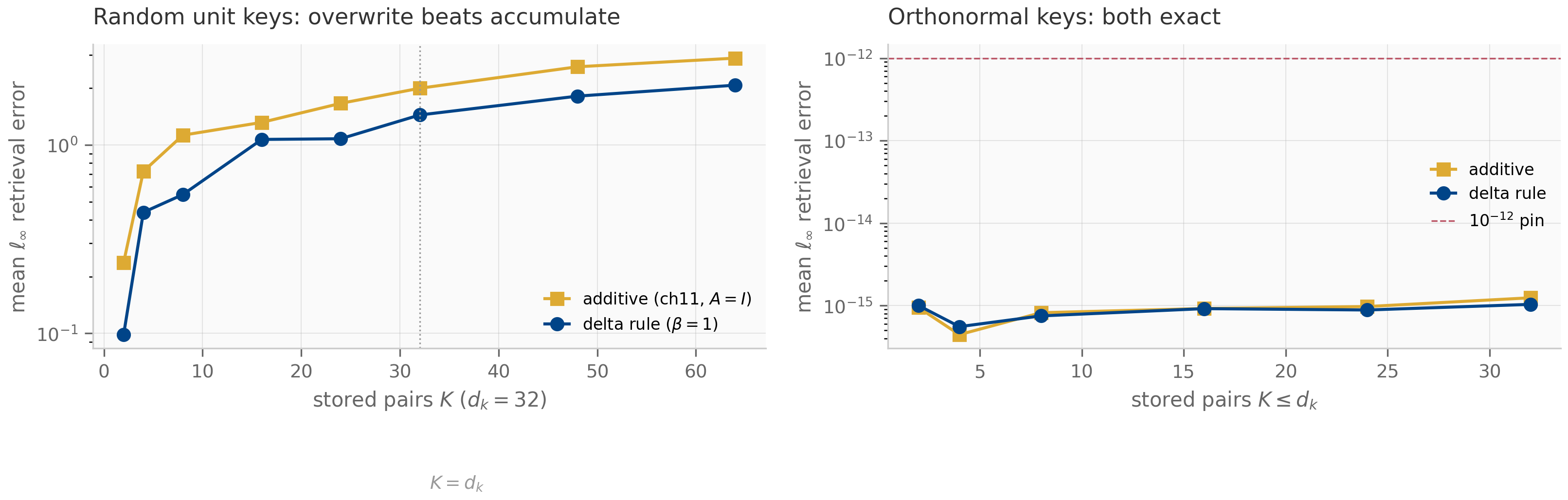
The figure is deliberately honest about the limit. With orthonormal keys both rules are exact — the delta rule’s advantage is zero when keys do not overlap — and with random keys both error curves still grow as passes : a rank- state cannot hold more than independent associations no matter how cleverly it writes (Proposition 11.4 still binds). The delta rule answers Chapter 11’s interference problem and its staleness problem (the overwrite), not the capacity bound. That distinction is exactly where Chapter 13’s matrix-memory architectures and Chapter 14’s hybrids will pick up.
12.3 Longhorn: the implicit step
Forward Euler is not the only one-step method, and Chapter 6 taught the alternative. Longhorn Liu et al. (2024) reaches it from the optimization side: frame the update as amortized online learning and solve, at each step, the regularized problem
a trust-region (proximal) step: improve recall on the incoming pair, but do not move far from the state you have. Setting the gradient to zero gives
Read the right-hand form against §12.1: this is the recall gradient evaluated at the endpoint , with step size — the backward-Euler step on the recall flow, the implicit method of Chapter 6.
An implicit equation usually costs a solve. Here the solve is free:
For the backward-Euler equation above has the unique solution
i.e. the implicit step is the delta rule evaluated at the self-limiting rate . In particular and for every key, however large.
The proof (Exercise 12.4, §12.9) is the classic implicit-solve move: right-
multiply the stationarity equation by , solve the resulting scalar
equation for the post-update prediction , and substitute back. In the
companion the identification is structural — longhorn_step simply is
delta_rule_step evaluated at — so the closed form gets
an independent certificate instead: solving the stationarity system
by dense linear solve
(no code shared with the rank-one form) reproduces it to ,
and the closed form zeroes the stationarity residual to
(pinned in
tests/test_longhorn.py::test_closed_form_equals_dense_implicit_solve).
Explicit and implicit methods
on this flow live in the same parametric family — they differ only in how the
effective step size responds to the data. DeltaNet’s is whatever the
network learned to emit; Longhorn’s self-adapts to the
key magnitude. Scaling the key by pushes the product
to ; by , to — approaching but provably never reaching . That
denominator is the entire difference between the two architectures, and §12.4
shows it is exactly the difference between conditional and unconditional
stability.
12.4 Stability regions: the explicit/implicit dichotomy
Both updates iterate an affine map in , so no linearization is needed: with and , a step at the (for now, repeated) pair gives exactly
The iteration matrix is a rank-one perturbation of the identity; its spectrum is immediate.
The matrix has eigenvalue in the direction and on the orthogonal complement. The deviation therefore contracts in the only direction the update touches iff , and:
- DeltaNet (explicit, ): stable iff . Past the boundary the deviation alternates sign and grows geometrically — forward Euler leaving its stability interval, Chapter 5’s picture replayed.
- Longhorn (implicit, ): for every and every key. Unconditional stability — the backward-Euler guarantee of Proposition 6.1, transferred to the online-learning flow. Moreover as : the hardest writes are the most strongly contracted, the L-stability signature.
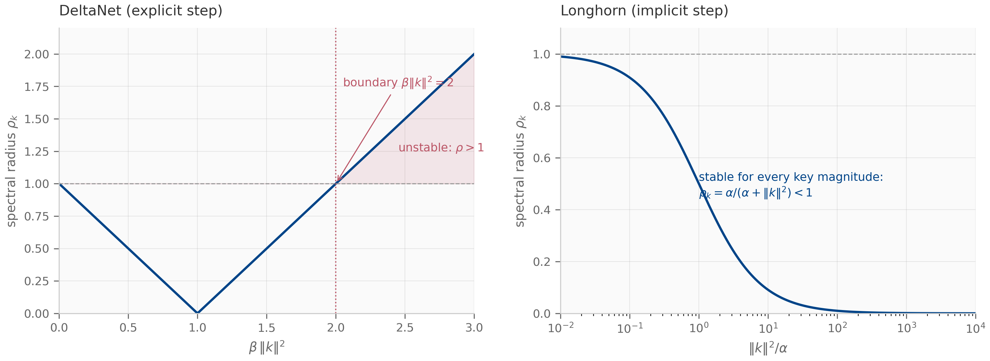
Because the deviation recurrence is exact — not a linearization — the geometric law is measurable to machine precision. Starting from under a repeated unit-norm key, the per-step ratio measured from the companion equals the analytic radius to twelve digits: for DeltaNet at , for Longhorn at . The trajectories make the dichotomy visceral:
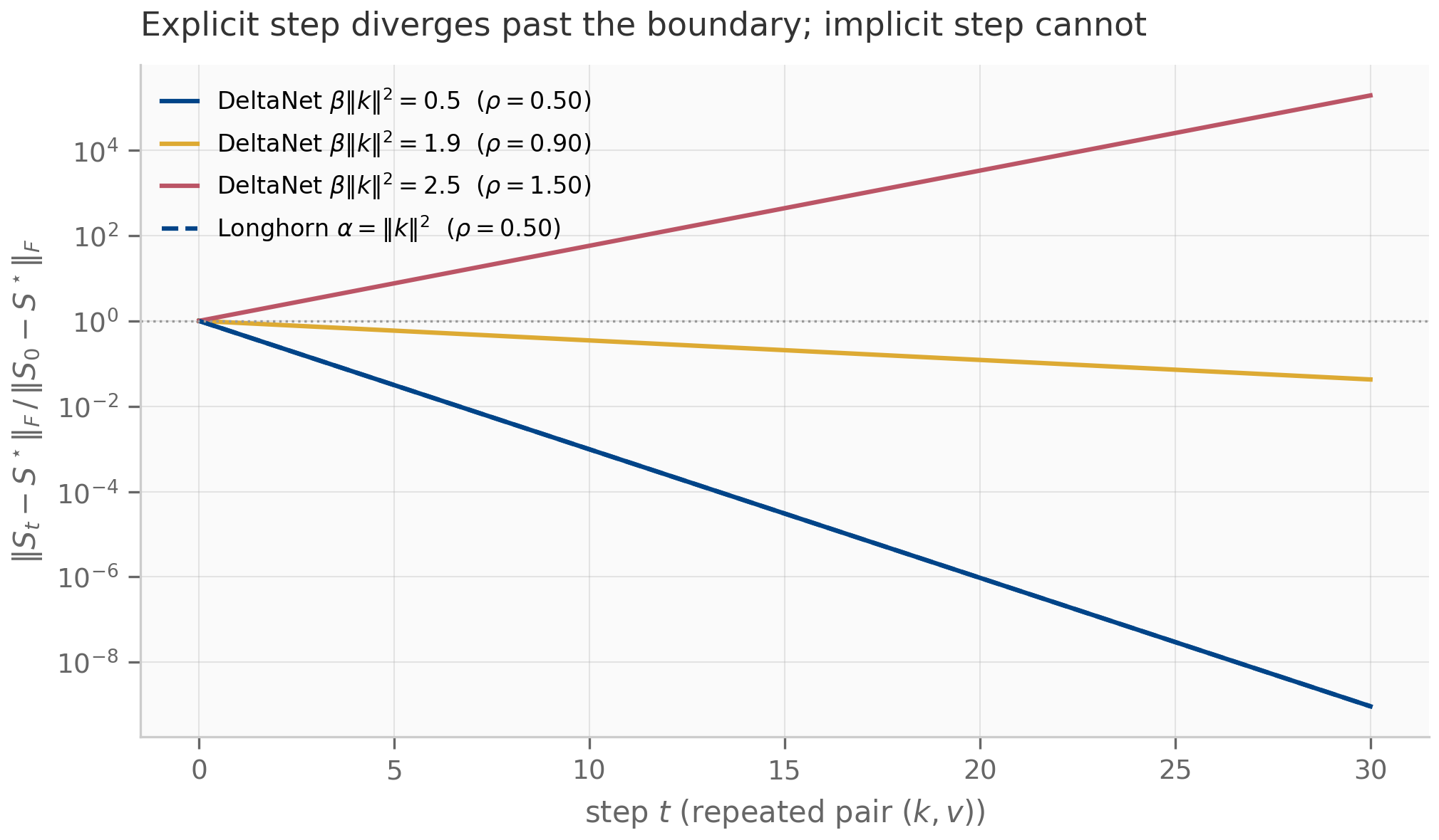
One degenerate-looking feature of Theorem 12.4 deserves emphasis: the orthogonal eigenvalue is exactly for both methods. Neither integrator forgets directions it has not been asked about — stability here is about the write direction only. Whole-state forgetting needs a different mechanism (§12.6).
Why trained DeltaNets are stable anyway. The dichotomy explains a design detail that looks cosmetic in the paper and is load-bearing in the lens: Yang et al. -normalize keys and parameterize Yang et al. (2024) . With that pins — not merely inside the stability interval but inside its monotonically-contracting half. And the per-step guarantee composes, which discharges the repeated-pair scoping above: with every factor has eigenvalues in , so the streaming product over any key sequence is non-expansive — the repeated pair is the worst case, not a special case. The architecture’s normalization choices are its stability guarantee, chosen at design time the way a step-size rule is chosen for an integrator. Longhorn needs no such guard, and that is precisely its selling point: stability by method, not by parameterization — the implicit-method trade Chapter 6 priced out, here with a free solve.
12.5 Chunkwise parallelization: the WY trick
The recurrent delta rule is sequential — fine for inference, hostile to training hardware. Chapter 11 met the same tension and resolved it with a second face of the same operator (Theorem 11.1); the delta rule’s resolution is the same move with one extra piece of numerical linear algebra. Split the sequence into chunks of size and unroll the erase-then-write form across one chunk:
with the chunk’s accumulated writes — the chunk’s own §12.2 recurrence run from a zero entry state, which is exactly how the companion materializes it. The cross-chunk recurrence is now one affine update per chunk ( sequential steps) and everything inside a chunk touches only chunk-local data Yang et al. (2024) . The remaining cost is the erase product — naively a chain of matrix products. But is a product of rank-one perturbations of , and numerical linear algebra has compressed exactly this object for decades:
For keys and rates , the chunk erase product admits the compact form
where the rows of are the keys and the rows of obey the recursion . Applying to a state is then two GEMMs, , never a materialized product chain.
The induction (Exercise 12.6, §12.9) is three lines. The companion pins both identities at machine precision on a stable-regime stream (unit-norm keys, — §12.4’s recommended operating point): the WY form matches the explicitly multiplied product to at worst across chunk sizes through , and the chunkwise driver — cross-chunk state passing with chunk-local sweeps — reproduces the monolithic recurrence bitwise (measured difference for every chunk size , because both run the same scan arithmetic in the same order). As in Chapter 11, the equivalence is the correctness certificate for the production form: one operator, two computation schedules.
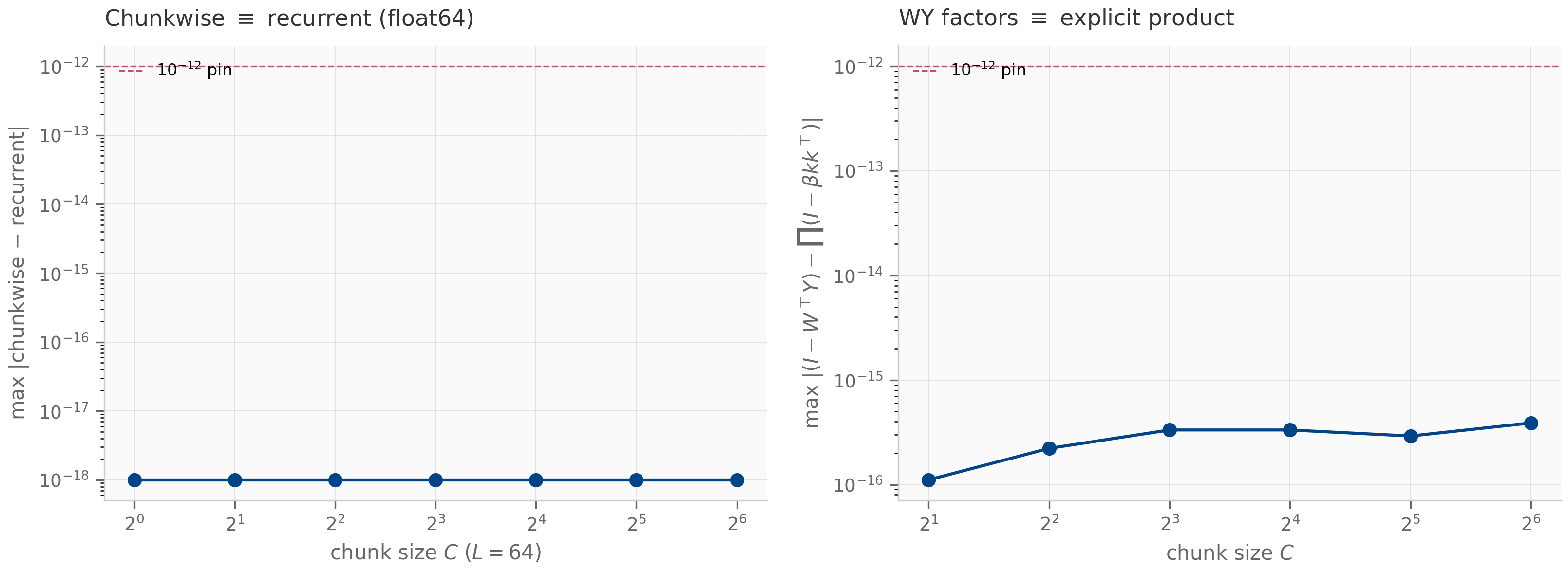
The practical punchline mirrors Chapter 11’s: the recurrent form is the inference mode, the chunkwise form is the training mode, and a fused kernel is an engineering refinement of an identity that is already exact in pure JAX.
12.6 Gating the delta rule: Gated DeltaNet and Kimi Linear
Theorem 12.4 left one direction untouched: everything orthogonal to the current key sits at eigenvalue exactly . A delta-rule memory never spontaneously forgets — stale bindings persist until their key is revisited. Chapter 9’s selective SSMs had the complementary skill: a scalar decay that forgets everything, uniformly. Gated DeltaNet Yang et al. (2025) composes the two:
The gate multiplies the erased state; the fresh write lands ungated. Both parents are exact limits, and the companion pins both reductions: recovers plain DeltaNet to , and is pure exponential decay — Chapter 9’s scalar-decay contraction with the carry promoted to a matrix, the same promotion Chapter 11 made for accumulation (Theorem 11.2).
The division of labor is exact, not approximate. Store a pair , then perform gated-delta writes whose keys are orthogonal to : the erase factors never touch the direction, so the retrieval decays only through the gate,
and the companion measures the product law at over forty writes. Gating forgets uniformly (a half-life for everything); the delta rule forgets selectively (exact overwrite of what is re-keyed). An architecture with both has independent control of the two timescales — which is why this update, not the plain delta rule, is what shipped. And the gate does not cost trainability: extending §12.5’s chunkwise/WY machinery to the -decayed erase product is a core contribution of the Gated DeltaNet paper Yang et al. (2025) , so the gated update trains with the same hardware efficiency.
That shipping lineage is current production history, summarized at architecture level. Kimi Linear Kimi Team (2025) builds its KDA (Kimi Delta Attention) layer as a refinement of exactly this gated update — the scalar replaced by per-channel diagonal gates, a finer-grained forgetting clock — and interleaves KDA with full attention at a 3:1 layer ratio, reporting up to a 75% KV-cache reduction at million-token contexts. As of mid-2026 this family — the gated delta rule adopted as the linear layer of public hybrid stacks, KDA in the Kimi Linear release — is the delta rule’s production form. This book derives the update those systems share; their layer-ratio and gate-granularity choices belong to Chapter 14’s hybrid design space, and the chapter makes no derived claims about KDA beyond the gated update above.
Step back to see the family whole. Chapter 9 proved selective SSMs and masked attention are one object (Theorem 9.5); Chapter 11 added the accumulation face; this chapter added the write-rule axis: accumulate (-write only), erase-and-write (delta), decay-erase-write (gated delta) — each one discretization choice on the same recall flow. Two limits now bracket the design space: the pure-decay limit (, an SSM forgetting on a slow clock) and the pure-write limit (attention-like immediate binding). Pilot B’s two-timescale benchmarks live exactly in that bracket — attention as the fast boundary layer, the decaying state as the slow manifold — and Chapters 14 and 16 build the architectures and the measurement protocol for it.
12.7 What’s next
This chapter closed Chapter 9’s “delta-rule lineage” promise and Chapter 11’s capacity hand-off: the write rule is now an optimizer step, and its stability theory is Chapters 5–6 applied to a new flow.
Two threads leave here open by design. Chapter 13 takes the lineage’s next generalization: RWKV-7’s generalized delta rule (transition rank-one in a learned direction, not the key itself) and xLSTM’s matrix memory with exponential gating — the gate moved inside the nonlinearity, with its own stabilization problem. Chapter 14 mixes these layers with attention into the production hybrids named above, where the layer-ratio and gate-granularity decisions we deferred become the design variables; Chapter 16 then builds the evaluation methodology — including the two-timescale protocol pilot B contributes — that makes the comparisons honest.
12.8 Exercises
Three short problems (solutions inline) and three longer ones (solutions in §12.9).
Exercise 12.1 (short)
With , unit key , and values , : compute the delta-rule state after writing then with , and the additive state for the same writes. Verify the retrievals are and respectively.
Solution
First write: . Second write: , so and : the old binding is gone. Additive: , retrieving — the stale residue of §12.2’s measured demo, by hand.
Exercise 12.2 (short, code)
Run companions/ch12/jax/delta_rule.py. Report the overwrite residuals and the
recall errors, then explain in one sentence why the orthonormal-key
panel shows both rules exact.
Solution
The script prints delta-rule overwrite residual against an additive stale residue of , and mean errors (additive) versus (delta). With orthonormal keys, every cross-term () vanishes, so the additive state already retrieves exactly and the erase factors act as the identity on all stored directions — there is no interference for the delta rule to remove.
Exercise 12.3 (short)
For and , compute Longhorn’s , the product , and the radius . Verify the complement identity and state what it says about where the “stable mass” goes as keys grow.
Solution
; products ; radii . Each pair sums to because exactly (the eigenvalue is positive here). As the write share approaches and the radius approaches : large keys are written harder and contracted faster — the L-stable behavior of Proposition 6.1‘s backward Euler, in optimizer clothing.
Exercise 12.4 (theory) — solution in §12.9
Derive Theorem 12.3: starting from the stationarity equation , obtain the closed form by solving for the post-update prediction first. Where exactly does get used?
Exercise 12.5 (theory) — solution in §12.9
Prove Theorem 12.4: compute the full spectrum of , derive the deviation recurrence from either update, and conclude the stability characterizations for both step-size rules. Explain why starting from makes exactly geometric rather than merely asymptotically so.
Exercise 12.6 (theory) — solution in §12.9
Prove Theorem 12.5 by induction on the chunk position, and count the cost of applying to a state via the WY form versus the materialized product, for chunk size .
12.9 Full solutions to theory exercises
Solution to Exercise 12.4
Right-multiply the stationarity equation by :
a scalar-shaped linear equation for the vector (the matrix unknown has collapsed because only appears). Since the coefficient is strictly positive — this is the only place positivity is needed, and it is what makes the implicit solve nonsingular for every key, including . Solve:
Substitute into the stationarity equation rearranged as :
Solution to Exercise 12.5
Spectrum. For any unit vector : , giving eigenvalue with multiplicity . For : , the single non-unit eigenvalue.
Deviation recurrence. Both updates have the form (Theorem 12.3 for Longhorn). Since ,
The affine parts cancel exactly — no linearization, no remainder.
Characterizations. Deviation components along (in the row space) are multiplied by each step; the component along is multiplied by . Convergence of the corrected direction requires , i.e. . DeltaNet’s free can violate this; Longhorn’s cannot, and directly.
Exact geometry from . Then , whose every row is a multiple of : the deviation starts entirely in the contracted direction, with no component on the eigenvalue- complement. Hence exactly — which is why the measured per-step ratios in §12.4 reproduce to twelve digits rather than only in the limit.
Solution to Exercise 12.6
Induction. Base : the empty product is , with empty factors. Step: assume where the rows of are . Then
The correction is rank one with row direction , so append and
which is the stated recursion, and .
Cost. WY application : one GEMM and one GEMM, total, plus the one-time factor build. The materialized product costs to build and to apply: for the WY route wins by a factor on both counts, and — the practical point — both of its operations are GEMMs, the shape hardware wants.
12.10 Companion code
The companions live in companions/ch12/{jax,torch,julia} and are float64
throughout. The JAX modules are canonical and produce all four figures; the
torch modules mirror the three operator updates with cross-framework parity
pinned to ; the Julia module ports the §12.4 stability analysis to a
third language using only the standard library, pinning the same closed forms
and trajectory ratios.
# JAX (canonical; emits the four figures to public/figures/ch12/)
PYTHONPATH=. python companions/ch12/jax/delta_rule.py
PYTHONPATH=. python companions/ch12/jax/longhorn.py
PYTHONPATH=. python companions/ch12/jax/stability.py
PYTHONPATH=. python companions/ch12/jax/chunkwise.py
PYTHONPATH=. python companions/ch12/jax/gated_delta.py
# Tests: JAX identities (< 1e-12), torch parity (< 1e-9), Julia stability suite
.venv/bin/pytest companions/ch12/jax companions/ch12/torch -q
julia --project=companions/ch12/julia companions/ch12/julia/runtests.jldelta_rule.py— the explicit step, its two algebraic faces, the fixed point, overwrite-vs-accumulate semantics, and the recall comparison figure (§12.1–12.2).longhorn.py— the implicit step via its closed form, verified against an independent dense solve of the stationarity system, plus the structural identity with the delta rule and the exact geometric error trajectories (§12.3–12.4).stability.py— the closed-form spectral radii, the named boundary, and the Rayleigh-quotient drift guard behind the stability-regions figure (§12.4).chunkwise.py— the WY representation, its two-GEMM application, and the chunkwise≡recurrent certificate (§12.5).gated_delta.py— the gated update, both exact reductions, and the uniform-forgetting law (§12.6). The torch mirror’s test file also documents the buffers-vs-Parameters distinction (a learned rate projection is a Parameter; a fixed rate floor is a buffer).
Exponential gates and matrix memory: xLSTM and RWKV-7
One generalized linear recurrence whose transition is diagonal-plus-rank-one — RWKV-7's generalized delta rule (rank-one removal in a learned direction, not the key) and xLSTM's matrix memory with exponential gating (and the log-domain stabilizer state that overflow forces) — extending Chapter 12's delta-rule lineage to matrix memories with their own stability questions.
Exponential gates and matrix memory: xLSTM and RWKV-7
13.1 The move: the gate inside the nonlinearity
Chapter 12 read a sequence layer’s state update as one step of an optimizer and organized the delta-rule family around a single linear recurrence,
with the state retrieved by and the transition acting on the right. Every architecture in that chapter shared one transition shape: — a scalar decay times the identity, minus a rank-one term locked to the write key . Gated DeltaNet’s was the only freedom beyond the delta rule, and it was a single number per step (Proposition 14.3 measures what that granularity costs).
Two threads were left open. Chapter 12 ended at the capacity wall (Proposition 11.4): a rank- state holds at most independent associations, and the delta rule erases interference without raising that ceiling. And its transition forgot only in the write direction — the orthogonal complement was inert, persistent memory that gradient flow on the current pair never cleans up. This chapter’s two architectures attack both by generalizing the transition itself, in two independent generalizations of the same linear recurrence:
- RWKV-7 Peng et al. (2025) keeps the rank-one shape but frees the removal direction and the diagonal: the erase direction need not be the key, and the decay is per-channel, not scalar. This is its “generalized delta rule,” and Chapter 12’s whole lineage falls out as a special case.
- xLSTM Beck et al. (2024) keeps a matrix memory and writes it with exponential gates — the input gate is , unbounded — which requires a stabilizer state to keep the recurrence inside float range.
The unifying object is the generalized transition
a diagonal decay (replacing Chapter 12’s scalar ) minus a rank-one removal in a unit direction (replacing the key-locked ). The rest of the chapter is two questions about this one matrix — when does it contract (§13.2), and what does freeing buy (§13.3) — followed by xLSTM’s exponential-gate variant and the stabilizer it forces (§13.4).
13.2 The generalized transition and its spectrum
Whether the recurrence keeps a bounded state is, as in Chapter 12, a question about the eigenvalues of the transition. The generalized is built from a diagonal and a symmetric rank-one term, so it is itself symmetric — and therefore has a real spectrum we can read exactly.
Let with a unit vector and . Then is symmetric, and:
- (Secular equation, interlacing.) Its eigenvalues are the for which , together with the roots of The rank-one downdate pushes every eigenvalue down without crossing the next diagonal entry, so the spectrum interlaces the sorted and lies in .
- (Scalar-diagonal case.) If , exactly one eigenvalue moves: the spectrum is , with spectral radius . At this is , recovering DeltaNet’s -direction radius (Theorem 12.4) under the identification — and the contractivity boundary is exactly forward Euler’s.
The proof is the matrix-determinant lemma: , so the roots of are the eigenvalues away from the
diagonal entries; the scalar case is the direct eigendecomposition of , whose only non- eigenvalue lies along (Exercise 13.4
carries the derivation). The companion reads the spectrum two ways — eigvalsh
of the materialized against the scalar-diagonal closed form — and they agree
to a measured ; the secular residual at the general-diagonal
eigenvalues is .
One reading of Proposition 13.1 matters for everything that follows. With a scalar diagonal at , the radius is : the transition is never strictly contractive, because the directions orthogonal to sit at eigenvalue exactly — Chapter 12’s inert persistent memory, unchanged. Strict contraction of those directions is what the diagonal buys: entries forget per-channel, the generalization of Gated DeltaNet’s single to a vector. Freeing the diagonal and freeing the removal direction are the two independent degrees of freedom RWKV-7 adds, and the spectrum shows they do different jobs — decay versus erasure.
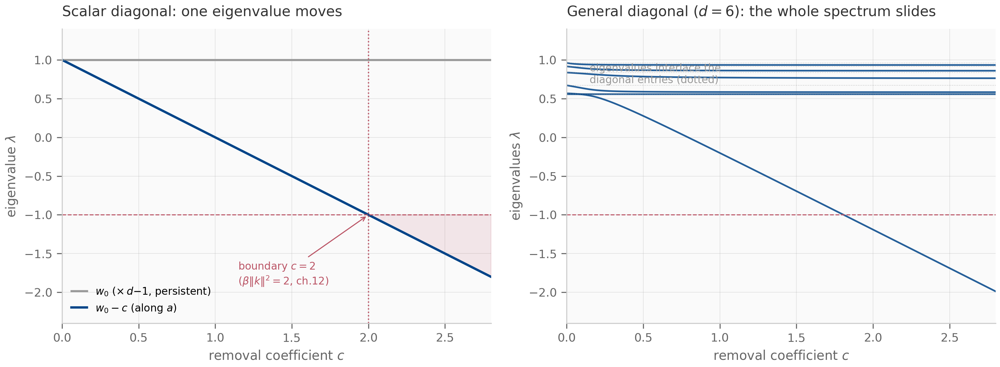
13.3 RWKV-7’s generalized delta rule
RWKV-7 Peng et al. (2025) runs the generalized transition over a stream,
with a per-channel decay , a unit removal direction , a removal coefficient , and a write whose key is decoupled from . The paper’s own framing is “a newly generalized formulation of the delta rule with vector-valued gating and in-context learning rates” — and the precise sense in which it generalizes the delta rule is a one-line reduction.
Set (scalar diagonal), (removal direction = unit key), , and write . Then the generalized recurrence equals Gated DeltaNet’s update
identically. Hence plain DeltaNet () and the entire Chapter 12 lineage are the scalar-diagonal, removal-locked-to-the-key special case; RWKV-7’s added freedom is precisely the per-channel diagonal and the learned direction .
The proof substitutes and matches: , and the scalar
diagonal contributes the , so (Exercise 13.5). The companion runs the
generalized recurrence with these parameters against Chapter 12’s
gated_delta_recurrent and pins the difference at ; the
rank-one lax.scan form matches the materialized-transition Python-loop oracle
at .
What does the learned direction buy, concretely? In Chapter 12 the only way to remove the association stored on a key was to write again with key — erasure was welded to the write. RWKV-7 can aim its rank-one removal at while writing some other, orthogonal pair, evicting the old association without overwriting it. Store on a unit key, then perform writes whose keys are orthogonal to :
- with the removal aimed at (direction , coefficient ), the retrieval decays as exactly — eviction with no overwrite;
- with the removal locked to the write key (Chapter 12’s ), the orthogonal writes never touch and — flat, the same inert-complement fact from §13.2.
The companion measures the decay at , as , matching to , against a flat locked baseline of . Decoupling the erase direction from the key is the whole content of “generalized” — and it is what lets RWKV-7 track state, not merely store associations.
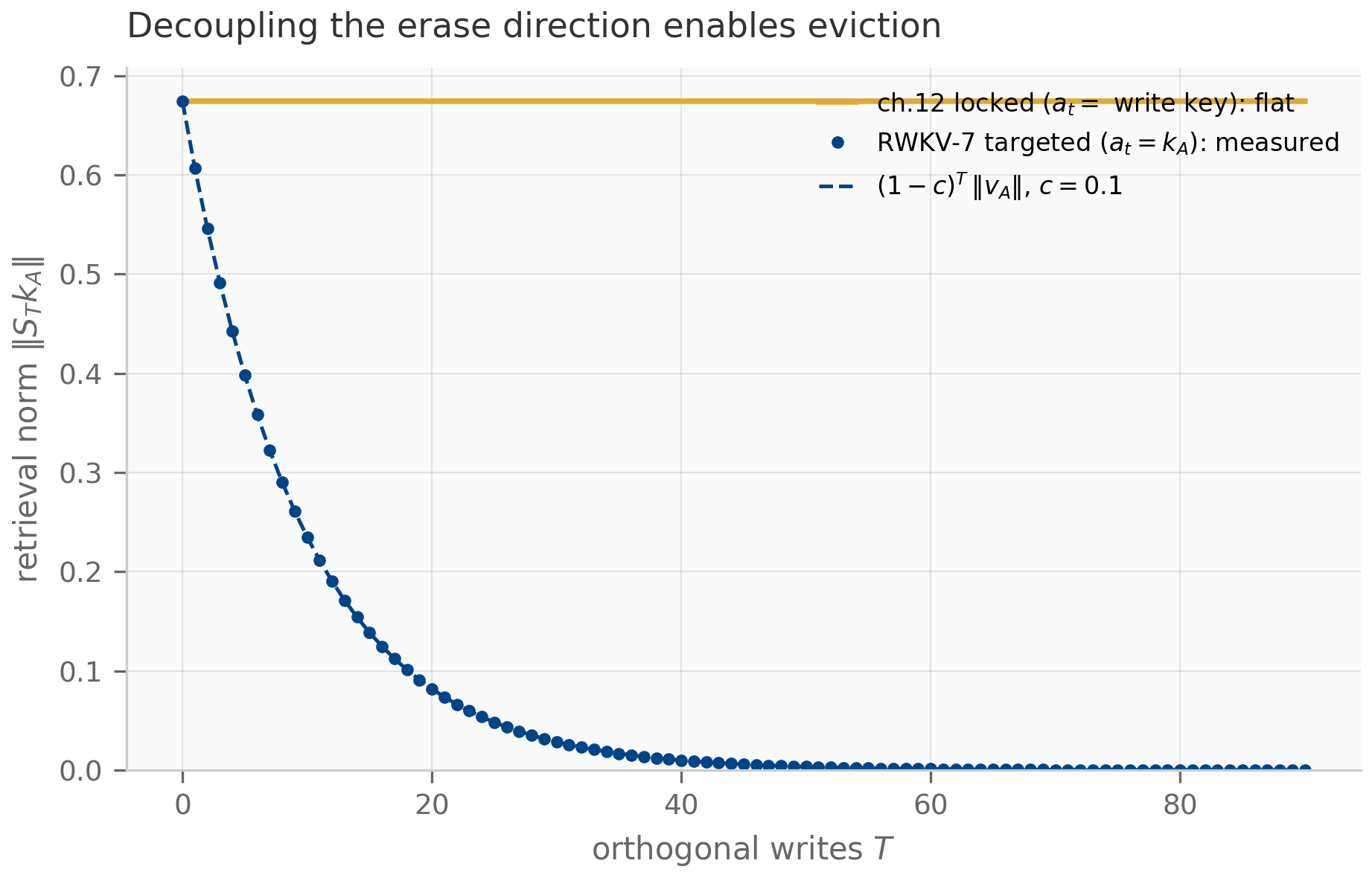
13.4 xLSTM: matrix memory and exponential gating
xLSTM Beck et al. (2024) arrives at the same matrix recurrence from the LSTM side rather than the delta-rule side. Its mLSTM cell carries a matrix memory and a normalizer vector ,
written with scalar gates the architecture moves inside an exponential: the
forget gate is bounded, but the input gate
is not. An unbounded input gate is the deliberate
move: it lets a single high-surprise token’s write dominate the entire running
memory — a sharper, winner-take-more selectivity than any sigmoid can express.
(xLSTM’s other cell, sLSTM, applies the same exponential gates to a scalar memory
with a memory-mixing recurrence; the matrix mLSTM is this chapter’s subject.) That
expressivity is exactly the source of the problem: overflows
float64 once , and the naive recurrence then produces
inf/nan.
The fix is a stabilizer state, a running maximum carried in the log domain:
with which the gates are rescaled and the memory is carried in scaled coordinates , . This is the online-softmax running-max trick, and it is exact:
Let be the naive mLSTM states with raw gates , , and define the stabilized states , via the max-state above. Then:
- (Range.) The rescaled gates and lie in (because and by definition of the max), so the scaled recurrence never overflows.
- (Exactness.) The readout is invariant under the rescaling: The only change is that the floor becomes . Wherever the naive recurrence is finite the two agree to machine precision; where it overflows, the stabilized one stays finite and still correct.
Part 1 is the definition of the max; part 2 factors out of numerator
and denominator (Exercise 13.6). The one place the rescaling is visible is the
readout floor — the constant becomes — and getting that scaling
right is exactly what makes the stabilizer a change of variables rather than a
numerical approximation: it buys range and costs nothing in the answer. The
companion confirms both halves: in the safe regime the stabilized and naive
readouts agree to ; pushed to an input log-gate of ,
the naive memory reaches a peak entry of — finite, but a
hair from the ceiling — and the readouts still agree to ; at
the naive recurrence overflows ( of its readout entries become
nan), while the stabilized one stays bounded (peak entry ) and exact.
The cleanest statement of what the stabilizer guarantees is a recovery property. Store one pair on a unit key with input log-gate , then read at : the stabilized readout is exactly , for any . With one write, and with , so — the normalizer cancels the gate, which is what the exponential input gate is for. The companion stores the fixed pair and recovers it to even at , where the naive recurrence has long since overflowed; the Julia companion recovers the identical value, a cross-language anchor on the stabilized readout.
This is the book’s stability thread reappearing inside the architecture. Chapter 2 asked when a state stays bounded; Chapters 5–6 answered it for integrators with the explicit/implicit dichotomy, and Chapter 6’s implicit methods bought unconditional stability by solving rather than extrapolating (Proposition 6.1). xLSTM’s stabilizer is the same bargain made numerically: it does not change which mathematical object the recurrence computes, it changes the coordinates so the computation stays in range — an unconditional guarantee that the matrix memory never overflows, paid for with one extra scalar of state.
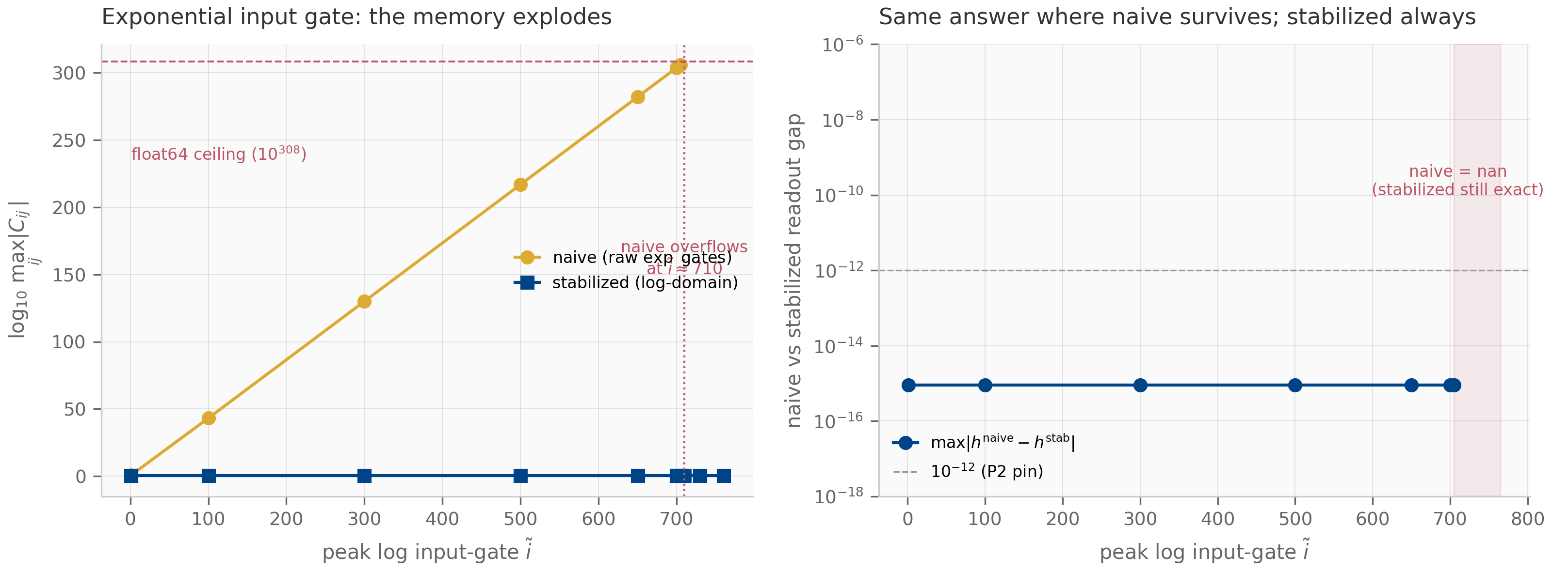
13.5 Stability, the trigger taxonomy, and the production lineup
Both architectures put a stability question inside the state — but in two different registers, and the difference is the point. RWKV-7’s is dynamical: the generalized transition contracts only when the diagonal decays and the rank-one removal stays within the boundary Proposition 13.1 draws — the explicit-method story from Chapter 12, now per-channel, a statement about the trajectory of the state. xLSTM’s is numerical: the exponential gate would overflow, and the max-state stabilizer is an in-state guarantee that it does not — not a claim about the dynamics at all, but about keeping the computation in float range, the implicit method’s unconditional-stability bargain made about representation rather than about the step. Chapter 15 returns to both with diagnostic tools (Lyapunov exponents, regime detection) that measure these stabilities on trained networks rather than asserting them at the architecture level.
There is a taxonomy worth closing here. Chapter 14 organized gates by what triggers a memory write — the input (content), the output, or a fixed layer schedule (Proposition 14.3). xLSTM’s exponential input gate is the sharpest input-triggered write in production. The remaining class is triggered by neither input nor position but by the model’s own loss: the Titans line Behrouz et al. (2025) writes to a neural long-term memory at test time, taking a gradient step on a surprise objective as it reads — a memory whose update rule is itself learned and fired by prediction error. That makes it a fourth trigger class (the loss), and it lives on a matrix memory of exactly the kind this chapter studies; its test-time-training mechanics are a distinct enough subject that this book names and places the trigger class here but does not pursue the test-time-training machinery further.
In production as of mid-2026 these are not toys: xLSTM has been trained at the B-parameter scale and RWKV-7 (“Goose”) at B, the latter reaching state-of-the-art multilingual performance at its size on dramatically fewer training tokens than comparable models Peng et al. (2025) . The diagonal-plus-rank-one transition and the exponential-gate stabilizer are not pedagogical simplifications — they are what these models run.
13.6 What’s next
Chapter 14 has already mixed these layers with attention into production hybrids, where the layer-ratio and gate-granularity decisions become design variables; Chapter 16 built the methodology that measures them honestly. The natural sequel to this chapter is Chapter 15, the counter-evidence file: it takes the stability questions raised here — when does a matrix memory’s recurrence stay bounded, and what can it provably not do — and turns them into diagnostics (Lyapunov exponents, effective state size) and impossibility results (the ceiling RWKV-7’s state-tracking claim brushes against). The generalized transition and the stabilizer state are the objects those diagnostics will probe.
13.7 Exercises
Exercise 13.1 (short)
For the scalar-diagonal transition (so , unit), use Proposition 13.1 to give the spectral radius at , , and . Which is non-contractive, and why is for every at this diagonal?
Solution
The spectrum is , so . At : . At : . At : — non-contractive (the iteration diverges, exactly forward Euler past its boundary). The radius is for every because the directions orthogonal to sit at eigenvalue : with the diagonal pinned at there is no per-channel decay, so the rank-one removal can shrink only the single direction . Strict contraction requires diagonal entries — the role of RWKV-7’s vector-valued .
Exercise 13.2 (short, code)
Run companions/ch13/jax/generalized_transition.py. Report the P3 reduction
error (generalized rule vs Chapter 12’s gated DeltaNet) and the decoupled-eviction
measurement at , : the targeted retrieval norm and the locked
baseline. What does the gap between them demonstrate?
Solution
The reduction error is — the generalized recurrence reproduces gated DeltaNet to machine precision, confirming Proposition 13.2. The eviction run reports targeted (matching to ) against a locked baseline of . The gap demonstrates the payoff of the learned direction: RWKV-7 can evict an old key by aiming its removal at it, while Chapter 12’s key-locked removal — under writes orthogonal to — leaves the association untouched. Decoupling the erase direction from the key is what “generalized” means.
Exercise 13.3 (short, code)
Run companions/ch13/jax/xlstm.py. Report the safe-regime readout gap between the
naive and stabilized recurrences, and the single-pair recovery error at input
log-gate . Why is the recovery error not affected by the gate’s magnitude?
Solution
The safe-regime readout gap is (the change-of-variables
exactness of Proposition 13.3), and single-pair recovery at
returns the stored value to — even though
overflows float64 and the naive recurrence is nan there. The
magnitude does not matter because the readout is a ratio: a single write makes
and with the same rescaled gate ,
and reading at gives . The
normalizer cancels the input gate exactly — which is precisely what an
unbounded input gate needs in order to be usable.
Exercise 13.4 (theory) — solution in §13.8
Prove part 1 of Proposition 13.1. Using the matrix- determinant lemma , derive the secular equation for the eigenvalues of away from the diagonal entries, and specialize to to recover the scalar-diagonal spectrum.
Exercise 13.5 (theory) — solution in §13.8
Prove Proposition 13.2. Substitute , , , into the generalized recurrence and show term-by-term that it equals Gated DeltaNet’s update. Identify which special case recovers plain DeltaNet, and which two degrees of freedom RWKV-7 adds over it.
Exercise 13.6 (theory) — solution in §13.8
Prove Proposition 13.3. (a) Show from the definition of . (b) By induction, show and where are the raw-gate states. (c) Conclude the readout identity, and explain why the constant floor must become rather than staying .
13.8 Full solutions to theory exercises
Solution to Exercise 13.4
Write and fix , so is invertible. Apply the matrix-determinant lemma with , , :
Since for , the eigenvalues there are exactly the roots of . (A diagonal entry is itself an eigenvalue iff , with eigenvector ; then the -term drops out of .) On each interval between consecutive distinct , is continuous and strictly monotone with poles of opposite sign at the endpoints, giving exactly one root per gap — the interlacing — and because shifts so that all roots lie at or below the corresponding , the spectrum sits in .
For : . Any vector orthogonal to is an eigenvector with eigenvalue (the rank-one term annihilates it), giving multiplicity ; and itself is an eigenvector, since . So the spectrum is and . At , , equal to once pushes the moving eigenvalue below ; with this is DeltaNet’s in the write direction, and exactly when .
Solution to Exercise 13.5
The generalized recurrence is . Substitute the four assignments. The diagonal term is . The rank-one term is
so . The write term is . Adding gives
which is exactly Gated DeltaNet’s update (Theorem 12.4). Setting (equivalently ) recovers plain DeltaNet, . The two degrees of freedom RWKV-7 adds over the lineage are (i) the per-channel diagonal in place of the scalar — vector-valued forgetting, the strict-contraction lever of §13.2 — and (ii) the learned removal direction , which decouples erasure from the write key (§13.3).
Solution to Exercise 13.6
(a) By definition , so and . Hence and , so and . Both are positive (exponentials) and at most .
(b) Induct on . At , and gives , consistent with the convention that the first write () discards the empty initial state. Assume . Then
using , . The identical computation gives .
(c) Substitute and into the naive readout:
The floor must scale to : the constant inside the naive lives in unscaled coordinates, and factoring out of the denominator divides it down to . Keeping the floor at in scaled coordinates would change the readout whenever the normalizer is small — the floor is the one place the change of variables is visible, and getting it right is what makes the stabilizer exact rather than approximate.
13.9 Companion code
The companions live in companions/ch13/{jax,torch,julia} and are float64
throughout; the JAX modules are canonical, the torch modules mirror their scoring
paths with cross-framework parity pinned , and the Julia module
cross-checks the stabilizer.
jax/generalized_transition.py— the diagonal-plus-rank-one transition, its spectrum (eigvalshagainst the scalar-diagonal closed form and the secular equation, Proposition 13.1), the generalized delta-rule recurrence (rank-onelax.scanvs a materialized-transition Python-loop oracle), the exact reduction to Chapter 12’s gated DeltaNet (Proposition 13.2), and the decoupled-eviction demo. Producestransition-spectrum.pngandlearned-direction.png.jax/xlstm.py— the mLSTM matrix-memory recurrence, the naive (overflow-prone) and log-domain-stabilized forms, the change-of-variables exactness (Proposition 13.3), the overflow cliff, and the single-pair recovery anchor. Producesstabilizer-overflow.png.torch/{generalized_transition,xlstm}.py— eager mirrors of the scoring paths, pinned to the JAX outputs intorch/tests/test_ch13_torch.py.julia/xlstm_stabilization.jl— a stdlib-only cross-language check of the stabilizer: the same P2 exactness, gate boundedness, overflow behavior, and the single-pair recovery of at input log-gate .
PYTHONPATH=. python companions/ch13/jax/generalized_transition.py
PYTHONPATH=. python companions/ch13/jax/xlstm.py
make companion-jax-tests # all chapters' JAX suites
make companion-torch-tests # JAX↔torch parity
julia --project=companions/ch13/julia companions/ch13/julia/runtests.jlHybrid architectures and gating mechanisms
Hybrids read through the two-timescale lens — attention as the boundary layer (exact on fast, token-local structure), the decaying state as the slow manifold (compressed carried context), and composition and gate granularity as the design variables; with the production lineup as of May 2026, the MAD methodology, and the two-timescale benchmark seed for pilot B.
Hybrid architectures and gating mechanisms
14.1 Two limits of sequence modeling
Part of this book’s argument has been that attention and state-space models are not rival species but two corners of one family. Chapter 9 made that literal: a selective SSM is a masked linear-attention computation (Theorem 9.5). Chapter 11 priced the recurrent corner: a finite additive state can hold only so many associations before interference swamps retrieval (Proposition 11.4), and Chapter 12’s delta-rule lineage bought back capacity with smarter writes at the cost of a genuine stability analysis (Theorem 12.4). The attention corner has the opposite ledger: retrieval is exact at any range it can see, and the price is a cache that grows linearly with what it has seen.
The trade is not hypothetical; it is the explicit organizing axis of the recall-throughput frontier mapped by Based Arora et al. (2024) : architectures that fix state size give up recall, architectures that keep recall give up the -per-token decode that makes long generation cheap. Pure designs sit at the frontier’s ends. The production systems of §14.5 sit deliberately in the middle, and the question this chapter equips you to ask is why the middle is the right place — not as an engineering compromise but as a statement about the sequences being modeled.
The statement is statistical. Real token streams mix two kinds of structure: fast, token-local dependence — syntax, local copying, the bigram-scale texture a short context pins down — and slow latent structure — topic, style, the document-level regime that changes rarely but conditions everything. (This decomposition-by-capability is also field practice: it is the premise of the synthetic-probe methodology of Poli et al. (2024) and Arora et al. (2024) that §14.6 takes up.) A layer that is exact over a short window serves the first; a compressed state that persists serves the second. Neither serves both: the window forgets the regime the moment it scrolls past the evidence, and the compressed state cannot reproduce exact local interactions it never stored. That intuition — two statistical timescales, two architectural resources — is the chapter’s lens. The next section gives it a theorem in the continuous prototype, and §14.6 an exactly computable discrete counterpart.
14.2 The two-timescale lens
The continuous prototype for “fast and slow living together” is a singularly perturbed linear system: a slow variable and a fast variable whose own dynamics relax on a timescale ,
with Hurwitz (every eigenvalue in the open left half-plane — a stable fast subsystem, the timescale separation that defines the stiff regime Chapter 6 tamed with implicit methods; Proposition 6.1). Setting formally gives : the slow manifold, the surface on which the fast variable has equilibrated to whatever the slow variable is doing. What happens off the surface is the boundary layer: a transient, of duration , in which collapses onto the manifold.
Let , with Hurwitz, so that for some , . Define the deviation from the slow manifold . Then for every fixed horizon and every bounded initial condition, as :
- Boundary layer. — the fast variable reaches an neighbourhood of the manifold in time .
- Reduced dynamics. The slow variable tracks the reduced system , , with .
The proof is a change of variables and one Grönwall estimate. Differentiating along trajectories,
since . The first term contracts at rate ; the second is a bounded forcing of size on bounded trajectories. Variation of constants gives claim 1. For claim 2, substitute into the slow equation: , so the difference obeys with , and Grönwall bounds by a constant times , which claim 1 bounds by . Exercise 14.4 carries the scalar case through explicitly; the nonlinear generalization is Tikhonov’s theorem Kokotović et al. (1986) .
The theorem licenses a reading of the hybrid division of labour — the reading Chapter 12’s closing section previewed:
- Attention is boundary-layer machinery. Within its window it computes pairwise interactions exactly — no compression, no model of how the past decays — which is precisely what fast, token-local structure needs, and exactly what a regime transient needs at the moment the slow context shifts.
- A decaying state is slow-manifold machinery. It carries a compressed, -size summary forward — the manifold parameterization — and its forgetting rate plays the role of the timescale assumption: Chapter 9’s selectivity and Chapter 11’s decay masks (Theorem 11.2) are mechanisms for making that rate fit the data’s slow rate.
- A hybrid is a matching construction. Sequential stacks, parallel gated blocks, and interleaved layers (§14.3) are different ways of joining the two descriptions — different matching conditions, in the asymptotics vocabulary.
What this lens does and does not claim. The theorem above is a statement about linear fast–slow ODEs, and in §14.6 an exact discrete counterpart is proved for a filtering task. The architectural reading — attention boundary layer, decaying state slow manifold, hybrid matched expansion — is an interpretive map between idealized computations, not a theorem about trained networks: nothing here claims that a trained hybrid implements a matching condition, and no such result exists. The map earns its keep where it is testable: it predicts which restriction fails on which statistics, and §14.6 measures exactly that. Its third leg is weaker, and we say so: the lens supplies the two specialists, not yet a theory of the joint — it does not by itself predict which matching condition (sequential, parallel, gated) wins where. The one careful cross-vendor comparison available — Lee et al.’s finding that sequential hybrids win at short context and parallel hybrids at long context Lee et al. (2025) — is consistent with components that specialize as the map says, and it is precisely the kind of data a theory of the joint would have to explain. Consistency is evidence for a lens, not proof of a mechanism; we will say “the lens predicts,” never “the network performs asymptotic matching.”
14.3 The composition design space
Fix the two primitives the rest of the chapter mixes, in the exact form the companion implements: sliding-window attention — causal softmax attention in which position attends to positions — and a gated-decay SSM, the per-channel EMA recurrence
the diagonal skeleton of Chapter 11’s gated linear attention, kept minimal so that every composition claim below is checkable to machine precision. Three composition patterns cover the production space:
- Sequential: one primitive feeds the other within a block, or — the in-series pairing every stacked hybrid uses locally.
- Parallel-gated: both read the same input and a gate blends them, — the Hymba Dong et al. (2024) /GMU-style pattern, and the carrier of §14.4’s granularity question.
- Interleaved at ratio : a residual stack in which every -th block is attention and the rest are SSM — the layer-ratio pattern, the design variable Chapter 12 deferred here from Kimi Linear’s 3:1 choice Kimi Team (2025) .
One boundary needs drawing, because the literature cuts this space twice. Sequential here is a within-block statement (primitives composed directly, no residual between them); a repeating block pattern — Griffin’s two recurrent blocks then one local-attention block, Jamba’s one attention block per eight — is an interleave in this vocabulary, whatever its authors call it. Lee et al.’s sequential-vs-parallel dichotomy Lee et al. (2025) is the coarser cut: their “sequential” covers every design in which information passes through the primitives in series — all interleaves included — against parallel-branch designs. We keep the finer three-way split and map their finding onto it where it is used (§14.5).
The companion pins the algebra that makes these well-posed objects of study (measured printouts; the tests pin each identity below ): the band-masked windowed attention equals its per-position oracle to ; window is full causal attention (identical outputs, exactly); under constant input the EMA matches its closed form to ; and the parallel gate’s endpoint reductions are exact — returns the attention branch bitwise, the SSM branch.
Why does the ratio — rather than, say, the window alone — carry so much design weight? Because decode-time memory is the binding constraint at production context lengths, and the ratio sets it:
A stack of mixing blocks of width , of which are sliding-window-attention blocks (window ) and are gated-decay SSM blocks, carries decode-time state
independent of the sequence length . A pure full-attention stack carries , growing linearly in . Per block, the hybrid budget is linear in the attention fraction .
The proof is counting: each attention block holds a rolling key buffer and a value buffer; each SSM block holds its -float state. The companion refuses to leave it at arithmetic — it materializes the buffers and asserts the formula against their actual sizes. At a production-shaped configuration (, ), the measured totals are floats at ratio and at , against for full attention at — factors of and .
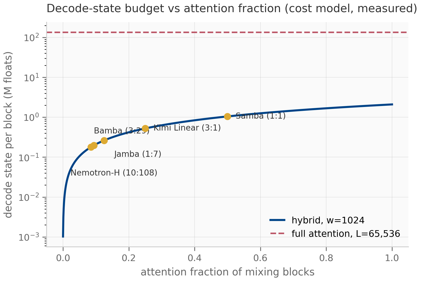
Two structural notes close the composition story. First, interleaving is the pattern that preserves trainability: every layer in the stack remains chunkwise-parallelizable — the SSM blocks by Chapter 11’s recurrent↔parallel duality and the delta-rule blocks by the WY machinery of Theorem 12.5 — so the ratio is a pure budget dial, not a training-throughput sacrifice. Second, the window and the ratio are not interchangeable: buys reach for the exact path, buys how often the exact path appears in depth. The two-timescale lens says their jobs differ in kind — must cover the fast structure’s correlation length, while the slow signal needs some carried state at some depth — and §14.6 measures exactly that asymmetry.
14.4 The gating design space
Composition decides where the two paths sit; gating decides, position by position and channel by channel, how much each path contributes. The production designs of §14.5 differ more in their gates than in anything else, and the differences organize cleanly along two axes.
Granularity — what shape the gate is:
Fix the two branch maps and consider parallel-gated blocks . The families
are nested as sets of realizable input–output maps, and each inclusion is strict under its own non-degeneracy condition: the first whenever the branches differ on at least two channels at some input; the second whenever the branches differ at two distinct inputs. Endpoints reduce exactly: gives the attention branch, the SSM branch; a -valued vector gate routes each channel to its branch.
The first strictness is a two-line argument: a vector gate that sends channel to attention and channel to the SSM would force a scalar gate to satisfy and simultaneously wherever the branches disagree on both channels. The second — input-dependent gates are genuinely stronger than constant ones — needs its two-input condition (a constant vector gate can already realize any single-input behaviour) and is Exercise 14.6. Both conditions hold generically for the actual attention/EMA branches. The companion pins the reductions and the channel-routing witness exactly (differences of , not merely small). The lineup also uses one coarser point on the same axis: block granularity, where the “gate” is the structural choice of which block type occupies which position — a routing decision made once, at design time, for a whole block.
The ordering is the cheap part; the design question is where on it to sit. A scalar gate costs one number and one design meeting; a vector gate is Chapter 11’s decay-mask vocabulary (Theorem 11.2) applied to branch mixing; input-conditioned vector gates are exactly the move selective SSMs made in Chapter 9, now steering the blend rather than the state. Production examples, as of May 2026: Nemotron-H mixes with a fixed schedule and no per-channel gate NVIDIA (2025) . Gated DeltaNet’s decay gate is the scalar per head Yang et al. (2025) — input-dependent but coarse — and Kimi’s KDA is precisely the per-channel (vector) refinement of it Kimi Team (2025) , the granularity class Griffin’s RG-LRU also occupies De et al. (2024) . SambaY’s Gated Memory Unit is an element-wise (vector) gate whose value is computed from a shared memory stream — input-dependent — while its placement across decoder layers is a fixed structural choice Ren et al. (2025) ; the trigger axis below classifies the value, not the wiring.
Trigger — what the gate responds to. A gate can be set by position (a fixed schedule: every -th block, Hunyuan TurboS’s macro-block patterns Tencent Hunyuan Team (2025) ), by the input (every selective/gated recurrence above), or — the 2026 frontier — by the model’s own output state: AMOR invokes attention only at positions where prediction entropy crosses a threshold, reporting attention on roughly 22% of tokens with long-context stability Zheng & Shani (2026) . The trigger axis has a sharp theoretical caution attached: Basu’s analysis of content-based routing argues that mechanisms which avoid pairwise token comparison cannot route precisely (1–29% routing accuracy across recurrent, memory-bank, and bandit-style gates) — high-precision routing needs pairwise machinery, the representational ingredient cheap gates omit, though not necessarily full attention: the same paper constructs a 99.7%-accurate router from a rank-one pairwise projection at linear cost Basu (2026) .
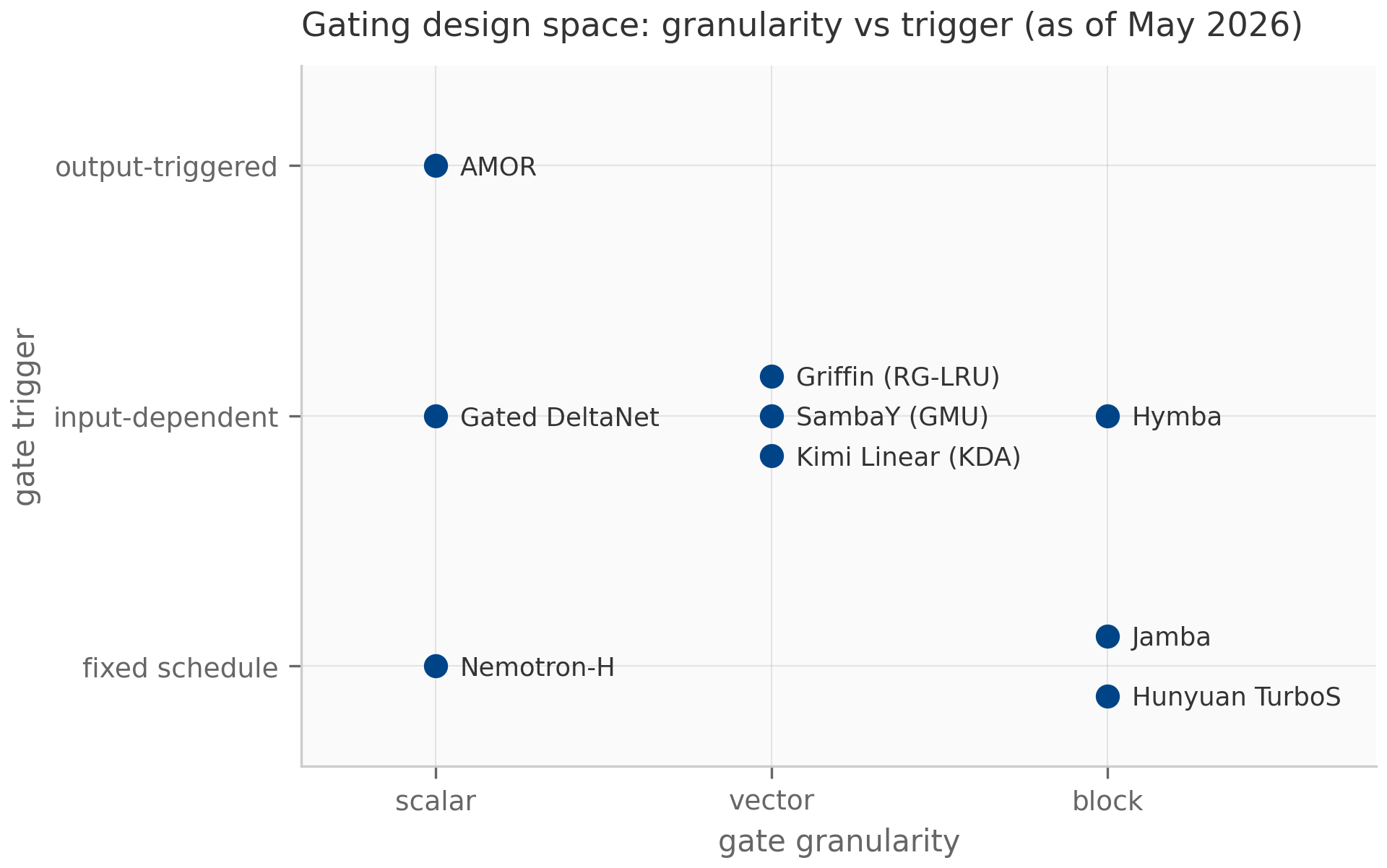
Two families that belong to this design space by shape are treated elsewhere: xLSTM’s exponential gates (granularity: vector; trigger: input; plus a stabilizer state the sigmoid families do not need) and the test-time memory writes of the Titans line (trigger: the loss, a fourth trigger class) are Chapter 13’s subjects, where their matrix-memory context lives.
14.5 The production lineup, as of May 2026
The lens and the design space were built to read a real lineup, so here it is. Mix pattern uses §14.3’s vocabulary; gate class uses §14.4’s.
| Model | Mix pattern (attention fraction ) | Gating | Reported headline (paper’s own) | |---|---|---|---| | Griffin De et al. (2024) | interleaved, 2 RG-LRU : 1 local attention () | vector, input-dep. | matches Llama-2 quality with faster long-sequence inference | | Samba Ren et al. (2024) | interleaved 1:1 Mamba + sliding window () | vector (Mamba’s) | linear-time training at 4K, length extrapolation to 256K context | | Jamba Lieber et al. (2024) | interleaved 1:7 attention:Mamba, MoE FFNs () | block-structural | 256K context at 12B-active scale | | Bamba (IBM, HF blog) Bamba Team (IBM, Princeton, CMU, UIUC) (2024) | interleaved 3:29 attention:Mamba-2 () | block-structural | fully open data recipe; ~2.5× vLLM decode throughput vs comparable transformers | | Nemotron-H NVIDIA (2025) | interleaved, 10 attention of 118 layers () | scalar schedule | ~3× faster inference than similarly sized transformers at comparable accuracy | | SambaY / Phi-4-mini-flash Ren et al. (2025) | Samba self-decoder + GMU cross-decoder, single full-attention layer | vector (GMU) | ~10× decoding throughput on long-generation reasoning | | Hunyuan TurboS Tencent Hunyuan Team (2025) | AMF/MF macro-blocks (attention–Mamba–FFN), MoE | block schedule | top-10 LMSYS arena placement at 56B activated | | Kimi Linear Kimi Team (2025) | interleaved 3:1 KDA:full attention (MLA) () | vector, input-dep. | 75% KV-cache reduction, up to ~6× decode at 1M context |
Read the table against Proposition 14.2 and the figure that draws it: every row sits low on the attention-fraction curve, exactly where the budget argument says the cheap exactness should be spent. The within-family motion is also informative: Samba → SambaY replaces cross-attention with a gate (GMU) and gains its throughput from the gating design space, not from a new mixing pattern; Jamba → Bamba → Nemotron-H is a march down the attention fraction as the slow-path layers improved (Mamba-1 → Mamba-2 Dao & Gu (2024) ); Kimi reaches the same neighbourhood from the delta-rule side, with Chapter 12’s gated-delta machinery as the slow path.
One cross-vendor regularity deserves its own sentence. Lee et al., comparing sequential against parallel mixing across vendors and scales, find sequential hybrids stronger at short context and parallel hybrids stronger at long context Lee et al. (2025) — the single most design-relevant empirical fact in the lineup. (Their dichotomy is the coarser cut §14.3 reconciled: “sequential” there spans the interleaves above.) Per §14.2’s flag, it is a consistency check for the matching lens — the kind of regularity a theory of the joint would have to explain — not a verification of it.
14.6 MAD and the two-timescale benchmark seed
How should claims like the table’s be tested? Full-scale training runs answer with averages over everything at once. The mechanistic-architecture- design (MAD) methodology Poli et al. (2024) answers with small, synthetic, capability-isolating tasks — in-context recall, compression, copying — chosen so that performance on the probe predicts scaling behaviour of the full architecture; the MQAR family Arora et al. (2024) did the same for associative recall specifically, and Chapter 11 already used it to measure the capacity wall. This section contributes the probe the two-timescale lens calls for, and it is pilot B’s seed.
The task. A hidden Markov model with the two timescales built in:
- a slow regime with sticky transition — stay with probability , else jump uniformly ( the all-ones matrix);
- a fast process: given the regime, tokens follow a regime-specific bigram table, on a vocabulary of size ;
- an overlap dial : the tables interpolate between a shared table and regime-specific ones, , controlling how hard the regimes are to tell apart locally — measured by the mean per-token discrimination (the average pairwise KL between regime rows).
Because the model is known, every predictor below is exact — no training, no approximation other than the stated information restriction — so every claim is a computation, checkable to machine precision. The Bayes-optimal predictor is the HMM forward filter, and the companion validates it against a brute-force enumeration over every regime path — paths for the prediction at position , an independent code path that is only feasible on short validation instances (): maximum prediction difference .
Three restrictions mirror the architectural resources:
- window- (the attention idealization): the same Bayes computation, restricted to the last tokens with a uniform regime prior at the window edge — exact pairwise machinery, zero carried state. With it reproduces the full filter exactly (difference ).
- fixed-decay (the state idealization): the filter run with the mixing-to-uniform prior update — a compressed state forgotten toward uniform at a fixed rate, the EMA of §14.3 wearing filtering clothes.
- unigram (the slow-manifold-only idealization): regime tracking with each bigram row replaced by the regime’s stationary unigram — carried state, no fast structure.
The fixed-decay restriction is the one with a theorem in it:
For every and ,
entrywise. Consequently the fixed-decay filter with rate is the exact Bayes filter for the two-timescale task: a fixed-decay state model is optimal when its forgetting rate matches the regime’s switching rate, and every other fixed is the Bayes filter for a misspecified switching rate — strictly costly whenever the regimes are distinguishable at all (the measured V-shape below; in the degenerate identical-tables limit every ties).
The proof is two lines of algebra on the diagonal and off-diagonal entries (Exercise 14.5). The companion measures the identity at entrywise and the resulting prediction agreement between the matched-decay filter and the optimal filter at . This is the chapter’s sharpest statement of the slow-manifold half of the lens: gating is timescale matching. Chapter 9’s selectivity and Chapter 11’s decay masks let a model learn ; the theorem says what the target of that learning is, and the V-shaped mistiming cost below says what missing it costs.
What each restriction costs, measured. At the committed reference configuration (, , , , , burn-in , nats/token), the optimal filter achieves nats. The window-8 predictor pays an excess of nats; a fixed decay matched to the wrong rate ( where the truth is ) pays ; the unigram predictor pays — twenty times the window’s tax. Dropping the fast structure is catastrophic; carrying the wrong-decay state or a modest window is merely costly.
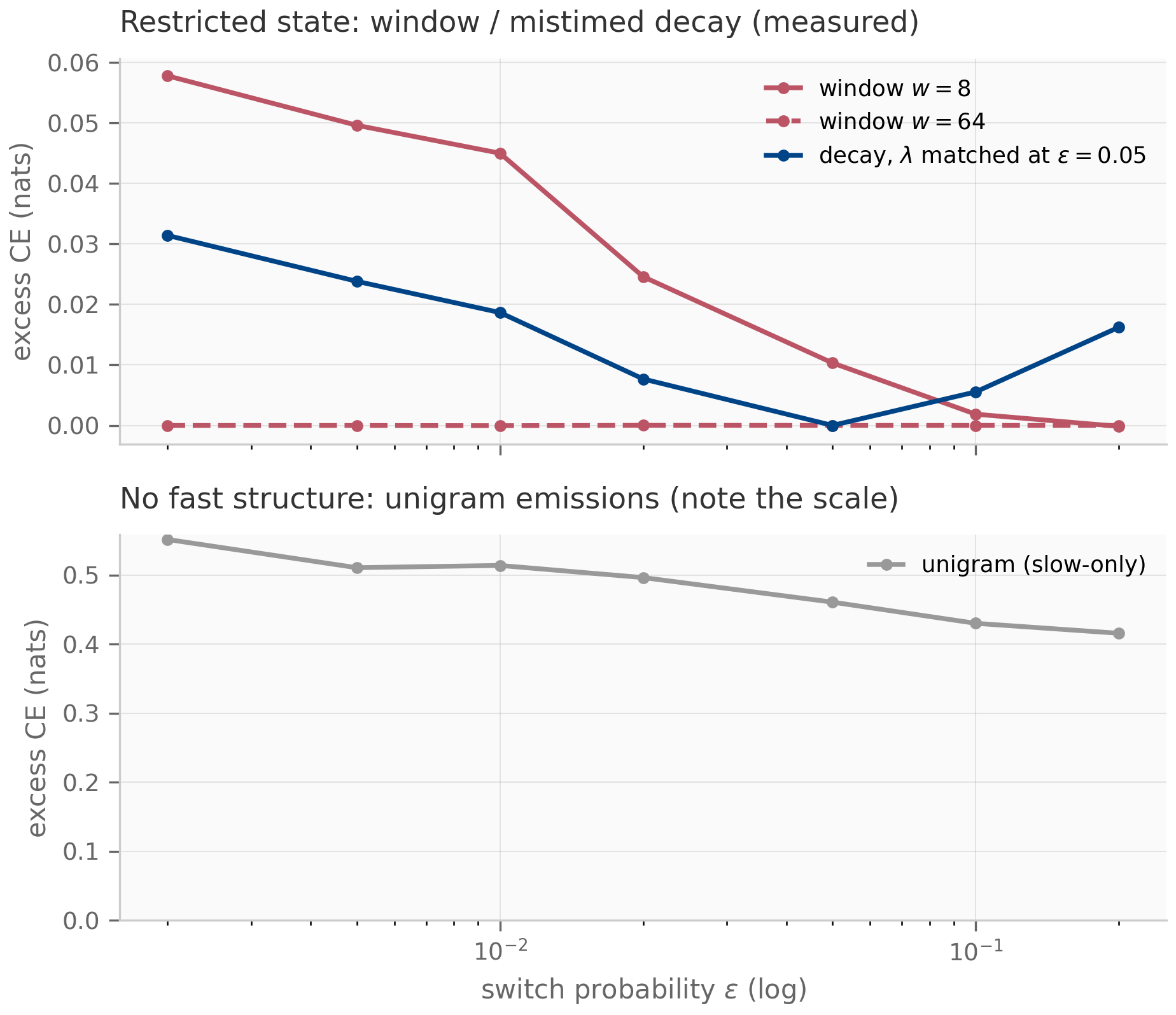
The third timescale, and the benchmark design lesson. The window curves above collapse to zero by . Why so small? Because with the regimes are still locally distinguishable enough that a few dozen tokens identify the current regime — the identification timescale is short. The overlap dial exists to control exactly this, and the crossover figure sweeps it:
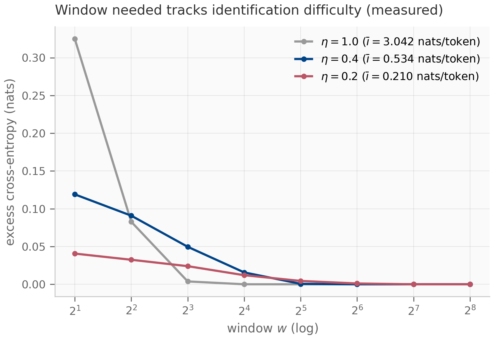
The design lesson is the section’s payload, and it is a constraint on benchmarks rather than on architectures: a two-timescale task separates fast-path from slow-path machinery only when the three timescales are ordered . Make the regimes too distinguishable () and a sliding window solves everything — the benchmark measures nothing about carried state. Make them too similar and even the optimal filter gains little — there is nothing to measure at all. Pilot B’s benchmark must therefore report (or place directly) as a task parameter alongside , exactly as this companion does. One measurement is deliberately deferred with the protocol: the composite restriction — a window- filter seeded at its edge with a decayed carried prior instead of the uniform one — is the idealized matched expansion itself, the natural probe of §14.2’s third leg, and it belongs with B’s protocol work rather than this chapter’s seed. What else does not transfer to Chapter 16 from here: the per-layer probing protocol that asks where a trained hybrid stores the regime posterior, the evaluation tiers around real benchmarks, and B’s five-axis decomposition — that is Chapter 16’s subject.
14.7 What’s next
This chapter mixed the layer families of Chapters 9–12 into hybrids and read the mixture through a fast–slow lens with one continuous theorem (Theorem 14.1) and one discrete one (Theorem 14.4) holding the interpretation to account. Its sibling beyond-SSM chapter, Chapter 13 (already behind you if reading in order), lives inside the gates themselves: exponential gating with its stabilizer states (xLSTM) and the generalized delta rule (RWKV-7) extend Chapter 12’s lineage to matrix memories with their own stability questions. Chapter 15 plays prosecution — the counter-evidence file on what SSM-heavy designs provably cannot do, and the diagnostic toolkit for detecting it. Chapter 16 builds the evaluation methodology this chapter’s benchmark seed feeds into — the protocol around the task, the per-layer probes, and the point where pilot B’s book-side prerequisites close.
14.8 Exercises
Three short problems (solutions inline) and three longer ones (solutions in §14.9).
Exercise 14.1 (short)
A 32-block hybrid has width , window , and ratio (so ). Using Proposition 14.2, compute the decode state in floats, the same stack’s full-attention cache at , and the ratio. At what context length does full attention’s cache equal the hybrid’s?
Solution
State floats. Full attention: — a factor of . Setting gives : past a few hundred tokens of context, this hybrid already stores less than full attention ever would.
Exercise 14.2 (short, code)
Run companions/ch14/jax/two_timescale.py. Report the reference-configuration
excesses (window-8, mistimed decay, unigram), then change _FIG_OVERLAP to
and to and report how the window-8 excess at
moves. One sentence: why does the hardest-to-identify task show the
smallest window-8 excess?
Solution
Reference: (window-8), (decay mistimed by a factor 10), (unigram). From the script’s printed crossover sweep, the window-8 excess at is at , at , at . Identification difficulty cuts both ways: at the regimes are hard to identify in a window, but knowing the regime is also worth less (the tables nearly coincide), so the achievable excess shrinks even as the window needed to remove it grows.
Exercise 14.3 (short)
Let and be the two branch outputs at one position, and suppose in every channel. Show that the set of outputs reachable by a scalar gate is a line segment in , that the vector-gate reachable set is the full axis-aligned box with corners and , and conclude the dimension counts ( versus ) behind Proposition 14.3.
Solution
Scalar: is the segment from to . Vector: channel of the output is , which ranges over the interval with endpoints independently of other channels — the product of nondegenerate intervals, i.e. the box. A segment is one-dimensional; the box is -dimensional, so for the inclusion is strict — and the corners of the box are exactly the channel-routing witnesses the companion pins.
Exercise 14.4 (theory) — solution in §14.9
Prove Theorem 14.1 in the scalar case , with : solve the dynamics exactly, exhibit the boundary layer, and bound on explicitly, identifying where each hypothesis (, fixed , bounded initial data) is used.
Exercise 14.5 (theory) — solution in §14.9
Prove Theorem 14.4, then compute the spectrum of and of , the stationary distribution of each, and the mixing time of the regime chain. Conclude that for large the matched rate : forgetting toward uniform at the switching rate.
Exercise 14.6 (theory) — solution in §14.9
Complete the second strictness in Proposition 14.3: construct two inputs and a target map realizable by an input-dependent vector gate but by no constant vector gate. Then explain why a gate computed from another layer’s state (the GMU pattern) sits in the input-dependent class.
14.9 Full solutions to theory exercises
Solution to Exercise 14.4
With the fast equation becomes, exactly as in the matrix case,
a scalar linear ODE with constant contraction rate (here is used — without it grows and there is no layer). Variation of constants:
On the trajectory is bounded uniformly in , say by — and this is where earns its keep a second time. Fixed horizon and bounded data alone give only an -dependent bound (the system matrix has entries); with , the contraction keeps , hence , the slow equation then bounds by an -independent Grönwall constant, and a standard bootstrap (pick dominating both estimates; continuity keeps the trajectory inside) closes the loop. Without the fast variable blows up as and no uniform exists. With in hand, , so the integral term is at most : the boundary-layer estimate , with the layer over by . Substituting into the slow equation gives , so obeys , , and
where the fixed horizon is used to keep the Grönwall factor a constant. Each piece of the theorem’s statement appears with explicit constants.
Solution to Exercise 14.5
The identity. Diagonal entries: and ; equality forces , i.e. . Off-diagonal: and , and at indeed . Both matrices are row-stochastic, so matching all entries matches the matrices; the constraint is . Since the Bayes filter’s only use of the regime chain is the prior update , replacing by changes nothing at any step: the fixed-decay filter at the matched rate is the Bayes filter, identically.
Spectra and mixing. Both matrices are of the form : eigenvalues on the all-ones vector and on its -dimensional complement. For : eigenvalue (stochasticity) and with multiplicity ; for : and . The stationary distribution of each is uniform (both are doubly stochastic). The regime chain forgets its initial condition at geometric rate per step — mixing time — which is the precise sense in which is the slow timescale. As , : forget toward uniform at exactly the switching rate.
Solution to Exercise 14.6
Take (one channel suffices) and any two inputs with and likewise . Define the target map to output the attention branch on and the SSM branch on . A constant gate must satisfy , forcing , and , forcing — contradiction. An input-dependent gate with , realizes the target, so the inclusion is strict. (With the same argument runs per channel.)
A GMU-style gate is computed from the hidden state of another layer — a deterministic function of the network input — so as an input–output map it is exactly an input-dependent vector gate: , with the cross-layer sharing changing where the gate’s information comes from (a memory stream computed once and reused) but not the function class. That is why SambaY’s throughput gain is a systems gain — fewer recomputations of expensive context — while its expressivity class is the one already characterized here.
14.10 Companion code
The companions live in companions/ch14/{jax,torch} and are float64
throughout. The JAX modules are canonical and produce all four figures; the
torch modules mirror the hybrid block and the filter family with
cross-framework parity pinned to (tokens drawn once and fed to
both implementations). No Julia module this chapter: the numerical core is
filtering linear algebra, not the integrator analysis that earned Julia its
seat in Chapters 10 and 12.
# JAX (canonical; emits the four figures to public/figures/ch14/)
PYTHONPATH=. python companions/ch14/jax/hybrid_block.py
PYTHONPATH=. python companions/ch14/jax/two_timescale.py
# Tests: JAX identities (< 1e-12), torch parity (< 1e-9)
.venv/bin/pytest companions/ch14 -qhybrid_block.py— sliding-window attention with its per-position oracle, the gated-decay EMA and its closed form, the three composition patterns with exact gate reductions, the schedule, and the decode-cost accounting audited against materialized buffers; produces the cost-frontier and design-space figures (§§14.3–14.5).two_timescale.py— the two-timescale HMM with the overlap dial, the exact forward filter validated against brute-force path enumeration, the window / fixed-decay / unigram restrictions, the matched-decay identity at machine precision, and the discrimination diagnostic ; produces the two-timescale-error and window-crossover figures (§§14.2, 14.6). This module is pilot B’s seed artifact.torch/— eager mirrors of both modules plus the buffers-vs-Parameters distinction in a minimal gated-mix layer (the learned blend is a Parameter; the fixed decay rates are a buffer).
Counter-evidence and diagnostic tools: where SSMs fail
The prosecution's file — what fixed-state and SSM-heavy designs provably cannot do (the TC⁰ ceiling, the illusion of state, the copying separation) and the diagnostic toolkit that measures stability and capacity on real systems, from an architecture-agnostic information-counting bound through the Benettin–QR Lyapunov estimator and its resolution limit to effective state size as a regime diagnostic, all validated against known ground truth.
Counter-evidence and diagnostic tools: where SSMs fail
15.1 The prosecution’s file
Three earlier chapters filed their counter-evidence here. Chapter 13 closed by naming this chapter “the counter-evidence file: it takes the stability questions raised here — when does a matrix memory’s recurrence stay bounded, and what can it provably not do — and turns them into diagnostics and impossibility results.” Chapter 14 cast it as the prosecution to its own defense of hybrids. Chapter 16 left “the impossibility side of the story — what else fixed state provably cannot do” explicitly to “Chapter 15’s file.” This chapter discharges all three.
The lens the book has used — a sequence layer is a dynamical system, read through its state — obliges two kinds of counter-evidence, and they are different in character:
-
Impossibility. Some tasks are out of reach not for want of tuning but for structural reasons: a fixed-size state is an information bottleneck, and a parallelizable recurrence sits in a circuit-complexity class that excludes genuinely sequential computation. These are theorems about every model of a given shape, and the strongest of them — the ceiling, the copying separation — are deep results we cite and attribute, never re-derive (§15.2). The one impossibility we can prove in a page is a counting bound (§15.3); it is deliberately weaker than the cited theorems, and saying exactly how it is weaker is half its value.
-
Diagnosis. Impossibility says what no such model can do; it does not tell you where this trained model sits. For that you need instruments that measure a concrete recurrence: its stability (does the state stay bounded? — Lyapunov exponents, §15.4) and its usable memory (how many modes actually persist? — effective state size, §15.5). These are the numerical-analyst’s tools, and the discipline of the chapter is to validate each against a system whose answer we know by construction before trusting it on a system we don’t.
The boundary between the two threads is the boundary between cited and proven, and the chapter marks it everywhere: a result in a shaded box with an attribution is someone else’s theorem; a result in a numbered proposition with a proof (or an exercise pointing to one) is ours, and every number it claims is measured by a companion.
15.2 The expressivity ceiling: TC⁰ and the illusion of state
The deepest counter-evidence is complexity-theoretic, and it cuts both ways. A transformer with logarithmic-precision arithmetic and a state-space model are, to first order, in the same computational class — and that class is small.
The phrase “illusion of state” is precise: a recurrence that the associative scan of Chapters 8–9 parallelizes is, by that very parallelizability, confined to the shallow-circuit class. The state buys linear-time inference and a place to put memory; it does not buy sequential expressivity. This is the formal counter-weight to a claim Chapter 13 flagged and deferred: RWKV-7’s paper reports that it “recognizes all regular languages,” apparently reaching above the ceiling. The reconciliation is in the fine print — that result holds for a fixed network with precision and depth allowed to grow with the automaton, not within the uniform, fixed-precision regime the impossibility theorems assume.
The copying separation makes the abstract ceiling concrete. Of Jelassi et al. Jelassi et al. (2024) : a two-layer transformer copies strings of length exponential in its size, while a fixed-state recurrence is bounded by what its state can hold — “structural, not a tuning issue.” That structural bound is the one piece of the impossibility story we can prove ourselves, and §15.3 does.
15.3 The capacity bound: a counting argument
Chapter 11 proved a rank wall for linear attention (Proposition 11.4) and Chapter 16 measured a recall cliff for an exact-capacity slot model (Proposition 16.1). Both are instances of one architecture-agnostic fact: a finite state is a finite communication channel, and no amount of cleverness lets a channel carry more than its capacity.
Let a deterministic sequence model process inputs by a recurrence carrying a hidden state in a set representable in coordinates at bits each, so . Suppose a task requires the model, after reading a prefix, to answer queries whose correct answers differ across a family of prefixes that must be distinguished. If , then two distinct prefixes induce the same post-prefix state, and the model answers them identically — wrong on at least one. In particular, losslessly recalling length- sequences over an alphabet requires
The proof is pure pigeonhole (Exercise 15.4): the post-prefix state is a deterministic function , every later output factors through , and forces a collision. Specializing to verbatim copy, the length- strings must all be distinguished, giving .
Two things make this honest rather than impressive. First, it is weaker than the cited theorems: it bounds lossless recall by counting, where Jelassi et al. exhibit the separation empirically and Merrill et al. place it in a complexity hierarchy. A real model also fails below this bound — interference, finite training, and lossy encodings mean the usable capacity is a fraction of . The counting bound is the ceiling of the ceiling. Second, it is architecture-agnostic: Chapter 11’s rank- state (, with the bits of a stored coordinate) and Chapter 16’s -slot store are the two instances where the abstract becomes concrete, and the chapter derived each separately. Here they are one count.
The companion realizes the bound on Chapter 16’s slot model, where each of slots holds one token-pair, i.e. bits. The abstract budget then meets the lossless requirement exactly at , and the measured recall cliff sits there.
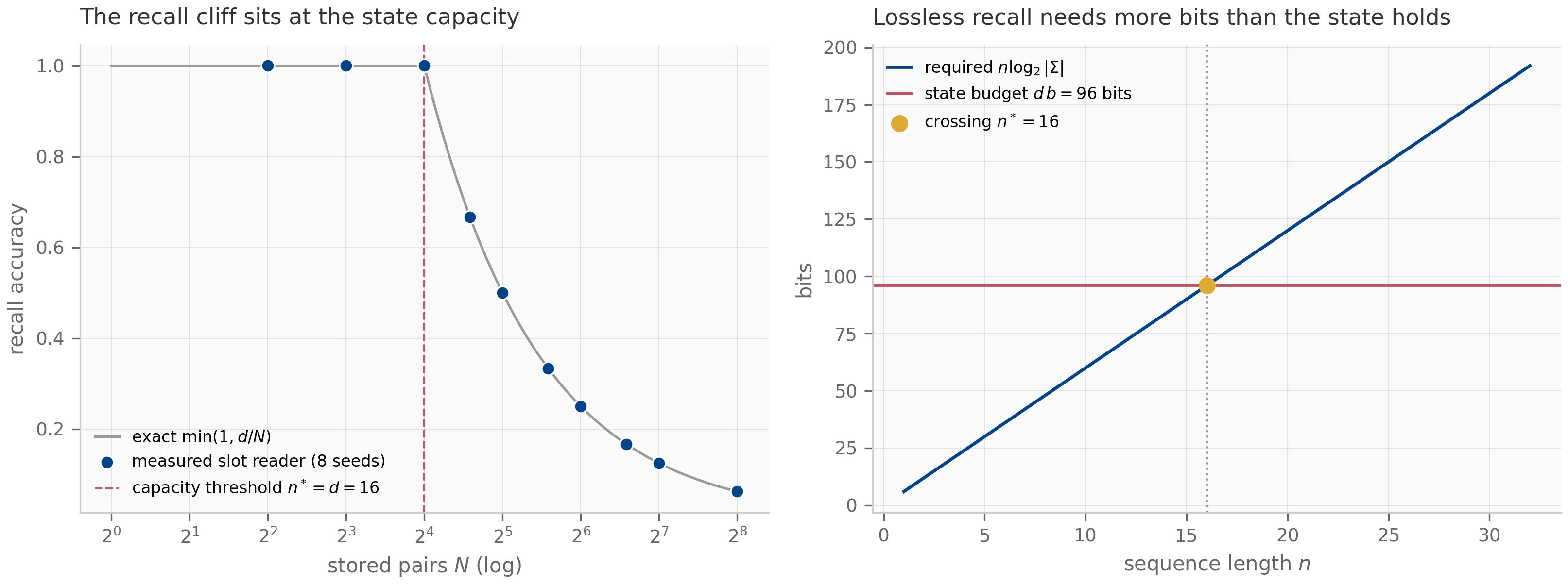
15.4 Lyapunov diagnostics: measuring stability on a concrete system
Impossibility is about all models; the rest of the chapter is about this one. The first instrument measures stability. Chapter 2 defined a system’s Lyapunov exponents as the asymptotic log-growth rates of its state (Definition 2.2, Theorem 2.1) and computed them with the Benettin QR algorithm Benettin et al. (1980) ; we reuse that engine unchanged and ask what it can and cannot tell us about a recurrence whose transition we did not choose — a trained-like SSM layer, the matrix memory of Chapter 13, a selective scan.
Let be the per-step Jacobian sequence of a recurrence, and let be the Benettin–QR estimate over a trace of length .
- (Recovery.) If the system is autonomous with a diagonalizable transition , then as ; the estimate is a time average, so its error decays like , and the top exponent (largest spectral gap) converges fastest.
- (Divergence identity.) For any and every , exactly, because the QR triangular factors satisfy . The sum of the exponents is the robust summary that survives even when the individual exponents do not.
- (Resolution limit.) When several modes share a modulus in a non-normal recurrence, the QR frame cannot isolate the individual exponents — they carry splitting noise — though their mean stays pinned by part 2.
Part 1 is the multiplicative-ergodic / QR-convergence theorem specialized to a constant map; part 2 is exact each step (Exercise 15.5); part 3 is the subtlety that matters in practice, and it is not about degeneracy alone. The companion makes the distinction sharp. A diagonal-plus-rank-one transition from Chapter 13 (Proposition 13.1), symmetric with distinct moduli, is recovered to a measured over steps (top exponent to — fastest, as promised); a diagonal selective/LTV Jacobian stream from Chapter 9 is recovered exactly (the decoupled coordinates make the QR trivial). Even a system that resembles an S4D-Lin layer at initialization — every mode decaying at the same rate , a degenerate spectrum — is recovered exactly, because its modes are decoupled.
The resolution limit appears only when degenerate modes are coupled: Chapter 2’s damped ring, a non-normal recurrence whose modes share a decay rate but rotate at different frequencies, scatters the per-mode estimates by a measured while the mean rate stays exact to . The lesson for diagnosing a trained model is concrete: trust the top exponent and the sum; distrust an individual interior exponent of a coupled system unless its modulus is well separated.
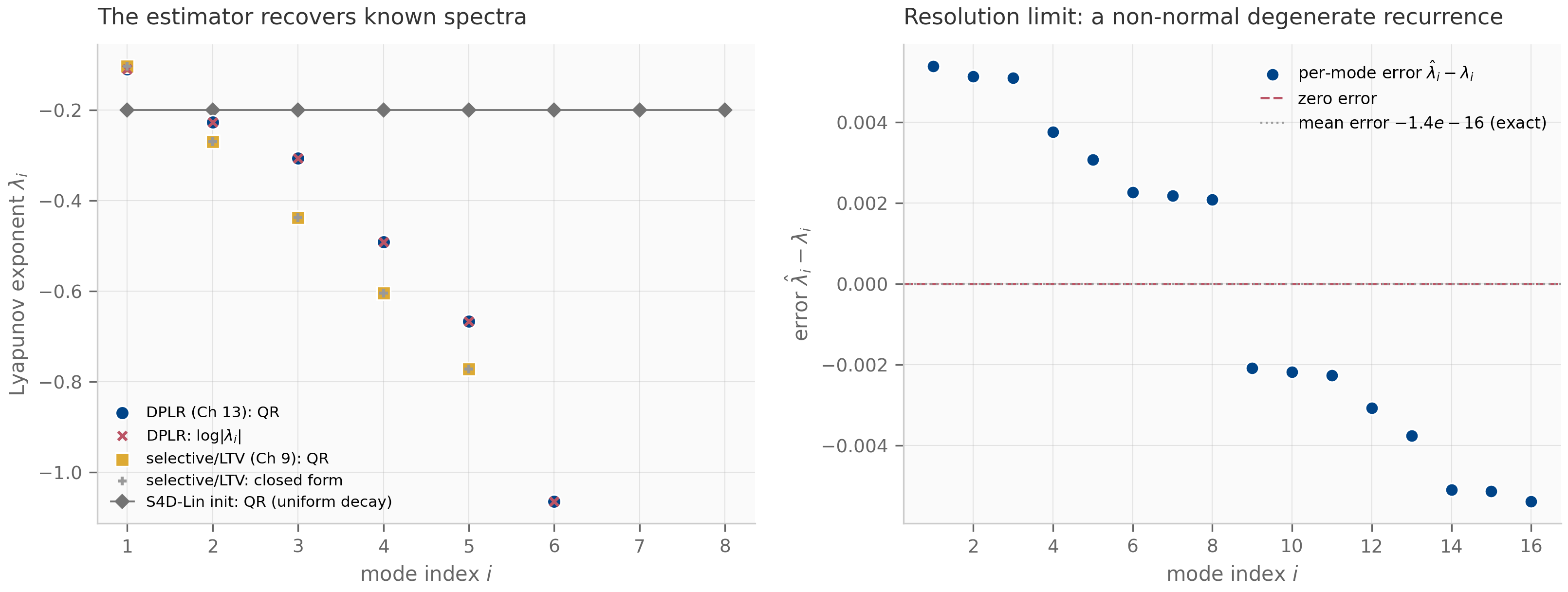
This is the diagnostic Chapter 7 anticipated — “the structure a stability or Lyapunov analysis of a trained S4 layer measures against” (Proposition 7.3) — and the one Chapter 2 named as the unified internal/input–output stability check, since an eigenvalue drifting toward shows up as a Lyapunov exponent crossing zero (Theorem 2.4). Running it on an actually trained network, where the Jacobian varies with the input and the modes are neither known nor decoupled, is pilot B’s program; the chapter validates the instrument, B points it at the data.
15.5 Regime detection and effective state size
The Lyapunov spectrum answers “is the state bounded?” The second instrument answers “how much of the state is actually doing memory?” A recurrence with coordinates may keep only a few of them near the marginal-stability boundary (persistent memory) while the rest contract quickly (transient). The count of persistent modes is the system’s effective state size, and it separates a memory regime from a forgetting regime.
Construct a transition with marginal modes () and contractive modes (). Then:
- (Two routes, one count.) The algebraic marginal count (from the eigenvalues) and the dynamical marginal count (from the Lyapunov spectrum) both equal for any slack separating the two levels. Independent computations — one algebraic, one dynamical — agree on the memory-mode count.
- (Effective state size.) With , the participation ratio is a continuous soft-count: as and as , interpolating between the marginal-mode count and the full dimension.
Part 1 is the anti-circularity guard that makes this a diagnostic rather than a tautology: an effective-dimension number “validated” by feeding it its own spectrum proves nothing, but two independent computations — the QR Lyapunov scan and the algebraic participation ratio — agreeing on a system whose is known by construction is real corroboration. The companion builds the system and confirms both routes return , with the measured participation ratio matching the closed form to ; the effective state size runs from at (nearly all memory in the marginal modes) to at (all eight modes comparably persistent).
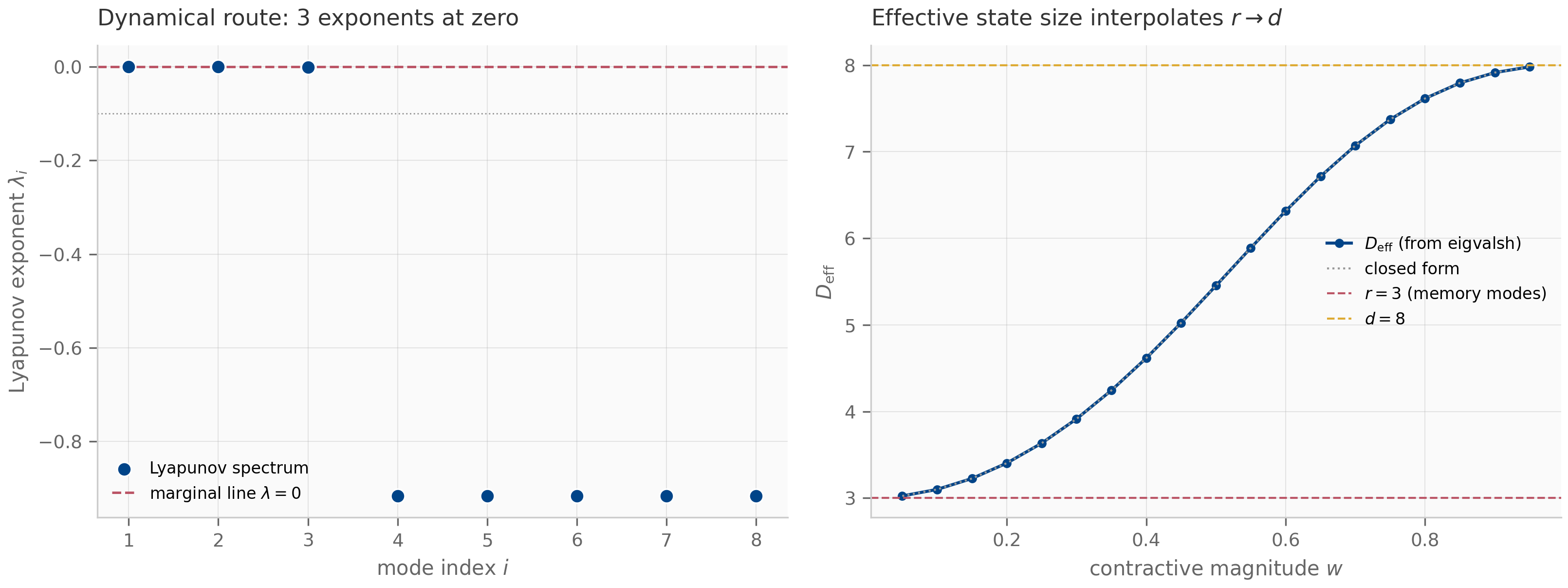
Effective state size is the diagnostic complement to the capacity bound of §15.3: the bound says how many bits a -coordinate state could hold; the effective size says how many coordinates a particular system actually keeps alive. A model can satisfy the capacity bound with room to spare and still fail on long-range recall because, after training, its has collapsed to a handful of modes. Measuring that collapse on trained checkpoints — across training, across layers — is, again, B’s empirical program; an independent Julia implementation of the same QR-Lyapunov algorithm (matching the JAX spectra on shared anchors — the diagonal and DPLR closed-form values — to ) guards the numerics the program will lean on.
15.6 The mechanistic verdict
The impossibility theorems and the diagnostics meet in a mechanistic question: when a recurrent model underperforms a transformer on recall, what fails? The sharpest counter-evidence here comes from the architecture’s own side. Of Bick, Xing & Gu Bick et al. (2025) — the last author is Mamba’s creator — the Gather-and-Aggregate mechanism: a few attention heads do the heavy lifting of in-context retrieval (a “Gather” head extracts the relevant span, an “Aggregate” head integrates it), and recurrent models, lacking the sharp content-based addressing those heads provide, produce a smoother, lossier read. That the sharpest critique of recurrent recall comes from the architecture’s own side motivates the hybrids of Chapter 14 rather than abandoning the line. This is mechanistic evidence, not a theorem — we cite it, and offer Chapter 16’s outer-product reader as the analytic stand-in for the limitation, not a reproduction of the finding.
It also bears on why Chapter 14’s hybrids win: the recall gap that Lee et al. (2025) traces in Mamba–transformer hybrids is the same gap G&A localizes to a few heads. A handful of attention layers supply the sharp addressing the recurrence cannot, and the diagnostics of this chapter — Lyapunov spectrum, effective state size — are how you would find, in a trained hybrid, which layers carry the persistent memory and which have contracted to transients.
The assembled toolkit is three instruments: the capacity bound (an upper limit no fixed state escapes), the Lyapunov spectrum (is the state stable, and which modes persist), and the effective state size (how many modes actually do memory). Each is validated here against a system with a known answer. None is run on a trained network in this chapter — that boundary is deliberate. Probing trained SSMs and hybrids with these tools is pilot B’s contribution, and deciding what the prosecution’s file and the defense’s together imply for architecture choice is Chapter 17’s synthesis.
15.7 What’s next
Chapter 17 integrates the pilots: it takes the diagnostics built here and the benchmark protocol of Chapter 16 and turns them on the C1 (symplectic) and B (two-timescale) programs, weighing the counter-evidence of this chapter against the fourteen chapters of construction that precede it. The instruments of §§15.4–15.5 are exactly what B carries to trained checkpoints; the impossibility results of §15.2 are the ceiling against which Chapter 17 reads any empirical win. Looking back, this chapter closes the stability thread Chapter 13 opened: the matrix-memory spectrum that chapter computed at the architecture level (Proposition 13.1, Proposition 13.2) is now a quantity a diagnostic measures on a concrete, possibly trained, system.
15.8 Exercises
Exercise 15.1 (short)
A diagonal SSM carries complex modes, each stored at bits, over a vocabulary . Use Proposition 15.1 to give the longest sequence it can losslessly recall. Why is a real model’s usable length strictly smaller than ?
Solution
The state budget is bits, and each token costs bits, so . A real model recalls fewer than tokens because the counting bound assumes a lossless, injective encoding of prefixes into states; a trained recurrence instead superposes writes (interference, the Chapter 11 rank wall), uses finite arithmetic, and never reaches the information-theoretic optimum. The bound is the ceiling of the ceiling — necessary, far from sufficient.
Exercise 15.2 (short, code)
Run companions/ch15/jax/lyapunov_diagnostics.py. Report the per-mode scatter and
the mean-rate error for the non-normal ring. What do the two numbers together tell
you about trusting a Lyapunov diagnostic on a trained (hence non-normal) recurrence?
Solution
The ring’s per-mode error scatters by while the mean rate is exact to . Together they say: on a coupled, non-normal recurrence with near-degenerate moduli, an individual interior Lyapunov exponent is unreliable (the QR frame cannot isolate it), but the sum/mean — pinned by the divergence identity — is trustworthy. On a trained model, read the top exponent (stability) and the sum (total contraction) confidently; treat an interior exponent as reliable only when its modulus is well separated from its neighbors.
Exercise 15.3 (short, code)
From the same run, report the two marginal-mode counts (algebraic and dynamical) and the effective state size at and for the system. Why does reporting both counts matter?
Solution
Both counts return ; the effective state size is at and at . Reporting both routes matters because they are independent: the algebraic count comes from the eigenvalues, the dynamical count from the QR Lyapunov scan. Their agreement on a system whose is known by construction is what certifies the diagnostic is measuring a real property rather than re-reporting its own input — the anti-circularity guard. A single route, agreeing only with itself, could be measuring an artifact.
Exercise 15.4 (theory) — solution in §15.9
Prove Proposition 15.1. Model the recurrence’s post-prefix state as a function , argue every later output factors through , and apply the pigeonhole principle when . Then specialize to verbatim copy to obtain .
Exercise 15.5 (theory) — solution in §15.9
Prove part 2 of Proposition 15.2 (the divergence identity). Using one Benettin step with orthogonal, show , and conclude for every , independent of any mode-resolution.
Exercise 15.6 (theory) — solution in §15.9
Prove part 2 of Proposition 15.3. For the two-level spectrum ( modes at , at ), derive from the participation-ratio definition, and take the limits and .
15.9 Full solutions to theory exercises
Solution to Exercise 15.4
Fix the suffix that poses the queries; then for each prefix the model’s answers are a deterministic function of the state it holds after reading (the recurrence is deterministic, and everything downstream sees only through ). So the entire answer map factors as . If , then cannot be injective (pigeonhole): there exist with , so the model produces identical answers on and . The task requires different answers on and (they are in , distinguished by construction), so the model is wrong on at least one. For verbatim copy, is all length- strings (each must be reproduced, hence distinguished), so losslessness forces , i.e. .
Solution to Exercise 15.5
One Benettin step orthonormalizes the propagated frame: with orthogonal and upper-triangular with the sign convention . Take determinants: . Orthogonal matrices have , and , so
The Benettin estimate is , so summing over and exchanging the sums,
This holds for every and uses nothing about whether the individual have converged or whether modes are degenerate — the sum is exact even when the per-mode split is not.
Solution to Exercise 15.6
With , the two-level spectrum has entries with and entries with . Then
so by definition
As the contractive terms vanish: , the marginal-mode count. As every : , the full dimension. For it lies strictly between and , a continuous interpolation — the soft count of usable memory modes.
15.10 Companion code
The companions live in companions/ch15/{jax,torch,julia} and are float64
throughout; the JAX modules are canonical, the torch module mirrors the diagnostic
core with cross-framework parity pinned , and the Julia module is an
independent-language Lyapunov cross-check.
jax/copying_bound.py— the information-counting bound (Proposition 15.1): the state-capacity and lossless-requirement bits, the recall-cliff threshold, and the demonstration that Chapter 16’s slot model (imported, not re-implemented) cliffs exactly at . Producescopying-bound.png.jax/lyapunov_diagnostics.py— the Lyapunov estimator (Proposition 15.2) reusing Chapter 2’sqr_lyapunov, the constructed systems (DPLR from Chapter 13, selective/LTV from Chapter 9, an S4D-Lin-like degenerate system, and Chapter 2’s ring for the resolution limit), the divergence identity, and the regime/effective-state-size diagnostic with its two-route cross-check (Proposition 15.3). Produceslyapunov-validation.pngandregime-separation.png.torch/lyapunov_diagnostics.py— an eager mirror of the diagnostic core (QR Lyapunov, closed form, effective state size), pinned to the JAX outputs intorch/tests/test_ch15_torch.py; the instrument is framework-agnostic because pilot B runs it on trained torch models.julia/lyapunov_crosscheck.jl— a stdlib-only independent QR-Lyapunov and eigendecomposition, matching the JAX spectra (diagonal recovery, the DPLR closed form) and the effective-state-size closed form to .
PYTHONPATH=. python companions/ch15/jax/copying_bound.py
PYTHONPATH=. python companions/ch15/jax/lyapunov_diagnostics.py
make companion-jax-tests # all chapters' JAX suites
make companion-torch-tests # JAX↔torch parity
julia --project=companions/ch15/julia companions/ch15/julia/runtests.jlEmpirical methodology: benchmark protocols and evaluation
Benchmarks as measurement instruments — the discriminative-regime principle for synthetic probes (tokenized MQAR with exact readers), length stress that pads with distractors rather than blanks (L90/AUC), the statistics of honest comparison (paired SEs, selection inflation), and the two-timescale protocol — composite predictor and probe signature — where pilot B's book-side prerequisites close.
Empirical methodology: benchmark protocols and evaluation
16.1 The measurement problem
This book has spent fifteen chapters arguing that sequence architectures are points in one design space, not rival species: a selective SSM is a masked linear-attention computation (Theorem 9.5), an additive state holds only as many associations as its rank allows (Proposition 11.4), smarter write rules buy capacity at the price of a stability analysis (Theorem 12.4), and a hybrid is a budget split between exact local computation and compressed carried state (Proposition 14.2). Every one of those claims ends in an empirical question: given two points in the design space, how do you tell which is better, and for what? Chapter 12 promised that the comparisons across its lineage would be made honest here; Chapter 14 handed over a benchmark seed and deferred its protocol. This chapter pays both debts.
The premise is that a benchmark is a measurement instrument, and deserves the same scrutiny as any other instrument: what quantity does it respond to, over what operating range, with what noise floor? The lens chapters tell us what the quantities are. A finite state has a capacity — so there must be a probe that loads it past capacity. Real streams have timescales — so there must be a task whose slow variable a window cannot see and whose decay rate a state must match. Exactness has a range — so there must be a stress that separates content the model must retrieve from content it may forget. And every one of these costs resources — cache, state, throughput — that the comparison must hold fixed or report. None of this is hypothetical: the synthetic-probe methodology of MAD Poli et al. (2024) and Zoology Arora et al. (2024) exists precisely because small tasks chosen this way predicted which architectures were worth pretraining.
What the lens does not supply is automatic validity. A probe can be solvable by machinery unrelated to its advertised quantity; a length stress can fail to stress anything; an evaluation can launder noise into a ranking. Each failure mode appears below with an exact, companion-checked example — including one we built by accident and kept as teaching material.
The chapter is organized as an evaluation stack with four tiers, numbered cheap to expensive: Tier 1 — mechanism probes, synthetic tasks isolating one capability, minutes to run (§16.2); Tier 2 — synthetic long-context stress with controlled length and timescale dials (§§16.4–16.5); Tier 3 — natural long-document suites, realistic but noisy (§16.4); Tier 4 — language-model quality and systems efficiency, the expensive anchor (§16.6). The statistics of §16.3 apply at every tier, and matter most where evaluation is noisiest.
16.2 Synthetic probes and the discriminative regime
A mechanism probe earns its keep by isolating one capability so cleanly that failure has a unique explanation. The Tier-1 canon, by target capability:
- associative recall — multi-query associative recall (MQAR): store key–value pairs, answer queries about them. The probe Zoology built, and the one Chapter 11 used to measure the capacity wall Arora et al. (2024) .
- in-context pattern completion — the induction-head task: attend to the previous occurrence of the current token and copy its successor Olsson et al. (2022) .
- selective copying — copy designated tokens while ignoring filler; the probe that motivated input-dependent selectivity Gu & Dao (2024) .
- string copying at length — reproduce an input verbatim. Copying a length- string means carrying tokens of information, so a fixed -dimensional state must fail once outruns its capacity while the attention cache grows with the input by construction; Jelassi et al. (2024) prove the separation in its strongest form — a two-layer transformer can copy strings of exponential length while fixed-state models are fundamentally limited by their state — which is the empirical face of Chapter 3’s Krylov-dimension reading of the recurrence’s expressive ceiling, and redeems that chapter’s promise here. The impossibility side of the story (what else fixed state provably cannot do) is Chapter 15’s file.
- composite suites — MAD’s six-task battery, used as a cheap screen whose scores rank-correlate with scaling behaviour Poli et al. (2024) .
Zoology’s central finding is that the language-model quality gap between efficient architectures and attention traces to associative-recall capability specifically — which is what made MQAR this tier’s anchor probe, and the reason the tier exists.
The companion builds the tokenized MQAR object end to end: episodes with disjoint key/value/filler alphabets, distinct keys, and every target key queried exactly once; ground truth defined by an independent scan oracle; and a family of exact readers standing in for architectures, in the same no-training discipline as §14.6 — each reader is an information restriction, so every curve below is a computation rather than an optimization outcome. The induction reader (exact-match attention reading the successor token — the Olsson et al. (2022) circuit as an analytic object) answers correctly at every load. The outer-product reader (the Proposition 11.4 mechanism on token embeddings) degrades smoothly past its dimension. And the slot reader — a ring buffer keeping the last pairs, abstaining on evicted keys — is the exact-capacity idealization, with accuracy exactly at load : the caricature of a fixed-size state with a hard edge.
The slot reader is deliberately simple, because simplicity is what makes the section’s design principle a theorem rather than a heuristic:
Let two readers keep the last pairs respectively, on episodes with distinct stored keys, each queried exactly once, evicted keys answered by abstention. Then each reader’s accuracy is exactly , so the accuracy gap
satisfies: for ; is increasing on , attaining its maximum at ; and decays to zero for . The probe separates the two capacities only for loads near — sized below the smaller state or far above the larger one, it measures nothing about the comparison.
The proof is four lines (Exercise 16.1 walks an instance). Exactly
of the queried keys remain in a last- buffer, and
abstention makes accidental correctness impossible, giving the accuracy
formula with equality; the three regimes of follow by cases on
, with monotonicity on because
increases in . The companion checks the accuracy identity at
rtol=0 — not approximately, exactly — and the gap curve below
peaks at at , is identically zero through
, and has fallen to by .
Two readings of the figure, one per direction of generalization. Soft readers shift, but do not escape, the principle. The outer-product reader’s gap peaks at , not : argmax decoding over value embeddings tolerates interference below a threshold, so the effective capacity sits above the raw dimension — but the gap still vanishes at small loads and still decays at large ones, and only the knee’s location moved. Calibrate the load to the mechanism actually under test, not to the nominal state size. The principle is Chapter 14’s lesson in a second coordinate. There, a two-timescale task separates window from carried state only when ; here, a recall task separates two capacities only when . Both are instances of one rule: report the dial that places the task in its discriminative regime ( there, here) as a first-class task parameter — a benchmark score without its dial setting is a number without units. The copying probe obeys the same rule: its dial is string length against state capacity, which is exactly why Jelassi et al. (2024) sweep length and why a copying score quoted at one length says little.
16.3 The statistics of honest comparison
Tier-1 probes are nearly noise-free — exact readers, exact oracles. Every tier above them is not, and two statistical failure modes account for a large share of unreproducible architecture comparisons. Both have exact antidotes, and both antidotes are cheap.
Pairing. Two predictors evaluated on the same items produce correlated scores: the items hard for one are mostly hard for the other. The honest uncertainty for a mean difference subtracts that shared difficulty; treating the two score sets as independent samples leaves it in.
Let be per-item scores of two predictors on the same items, with sample variances , sample covariance , and sample correlation . The standard error of the mean difference computed from the paired differences satisfies
where is the two-independent-samples formula. With equal variances the ratio is : at , pairing shrinks the standard error tenfold; ignoring the pairing overstates it tenfold.
The proof is the variance of a difference of correlated means (Exercise 16.4). The companion’s demonstration uses the §16.5 reference stream: the window-8 and composite predictors differ by nats of per-token log loss over shared positions, with per-item correlation . The paired standard error is ; the unpaired formula gives — larger. The same measured difference is a result with the correct statistic and an unpublishable with the wrong one. Pairing is not a refinement; it decides whether the experiment worked.
Selection. The second failure mode is quieter: evaluate variants — seeds, sweeps, ablation cells — and report the best. If the variants are equally good, the reported number still exceeds the truth by the expected maximum of noise draws.
Let be the evaluation-noise components of variant scores, each mean-zero and -sub-Gaussian (in particular, ). Then
Reporting the best of equally good variants therefore overstates quality by up to — a bias that grows without bound in , shrinks only through (more evaluation data), and vanishes only when the selection split is independent of the reporting split.
The proof is five lines with the moment generating function (Exercise 16.5). Measured on Gaussian draws, the expectation reaches at and at against bounds of and — the bound is conservative but the growth is real:
And measured in the wild: scoring embedding seeds of the same outer-product reader (identical true accuracy by symmetry) on the same -episode battery, the best seed beats the across-seed mean by accuracy — against a predicted from the measured seed spread . The theory prices the malpractice to within a rounding error.
The protocol consequences fit in three rules. Pair everything pairable: evaluate all variants on identical items and report paired SEs (per-token losses pair naturally; per-episode accuracies pair across shared episodes). Freeze the suite before the sweep: a task set adjusted after seeing results is a selection mechanism, and inherits the tax without disclosing its . Report the sweep, not its maximum: best-of- is legitimate model selection exactly when the selected model is re-scored on data the selection never touched — the held-out discipline every probe in this chapter applies, down to the ridge probe of §16.5 fitting on the first half of a stream and scoring on the second.
16.4 Long-context evaluation and length-robustness metrics
Tier 2 asks the question the lens cares most about: does the mechanism hold at separations it was not tuned on? The field’s instruments here have a cautionary history worth one paragraph. Long Range Arena Tay et al. (2021) defined the long-context battlefield of 2020–2022 — six classification tasks at lengths –K, culminating in Path-X — and S4 famously broke it open, solving Path-X for the first time ( Gu et al. (2022) ; Chapter 8’s kernel machinery is why it could). But LRA’s tasks are classification over long inputs, not recall, copying, or in-context use of long inputs — the capabilities that §16.2’s probes target and that language modeling actually exercises. As LTI SSMs saturated LRA while failing selective-copying and recall probes (the gap Chapter 9’s selectivity exists to close; Gu & Dao (2024) ), the field’s weight shifted to recall-centric instruments. The methodology lesson is not that LRA was a bad benchmark — it was a well-built instrument for its quantity — but that saturating an instrument retires it: past that point it ranks tie-breaking noise, and §16.3’s selection arithmetic takes over.
The current Tier-2/3 workhorses ask retrieval questions directly. Needle-in-a-haystack stress plants target content at controlled depths in long filler and queries it; RULER Hsieh et al. (2024) systematizes this with multi-key, multi-value, and aggregation variants at controlled lengths, and reports large gaps between claimed and effective context across model families — the single most protocol-shaped finding in the long-context literature: a context-window number on a model card is a claim about an instrument’s range, and RULER is the calibration. On the natural-document side (Tier 3), SCROLLS Shaham et al. (2022) and LongBench Bai et al. (2024) aggregate QA, summarization, and reasoning over real long documents — high validity, but noisy generative metrics (F1, ROUGE) at modest item counts, which is precisely where §16.3’s paired statistics earn their keep.
What should the synthetic version of length stress look like? The
companion answers with a negative control we hit by accident. Take the
fading-memory reader — the outer-product state decayed by per token,
the cleanest caricature of a fixed-rate forgetting recurrence — and stress
it by widening the key-to-query separation with neutral filler. Nothing
happens. Exactly nothing: every stored weight rescales by the same
, argmax decoding is scale-invariant, and the companion pins
prediction-level equality between gap and gap at rtol=0. A
NIAH-style stress built on blank padding measures nothing about fading
memory. What stresses it is fresher competing content: distractor
pairs written after the targets leave the target signal at
against interference that decayed far less. RULER’s
multi-key variants embody the same insight (the haystack is made of hay,
not vacuum); the companion makes it exact, and the design rule is pad
with content, not blanks.
The figure also separates two failure modes the single word “fails at length” conflates: the decayed readers fail by recency (the target faded), the undecayed one by capacity (the buffer filled) — same downward curves, different mechanisms, distinguishable because the generator controls and independently. That is the Tier-2 advantage over Tier 3 in one picture.
Curves invite single-number summaries, and the long-context literature’s single-number practice is worth formalizing. For a measured accuracy curve over a strictly increasing separation grid :
- — the longest separation retaining of short-range accuracy (the range of the instrument, in the calibration sense);
- — mean accuracy per octave of separation (trapezoid on the measured grid), rewarding robustness across scales rather than across raw tokens.
Both are implemented and exactness-tested in the companion
(hand-constructed curves, rtol=0), and both inherit §16.2’s caveat:
a single without its grid and task dials is a number without
units — report the curve, quote the summary.
16.5 The two-timescale protocol
Chapter 14 shipped pilot B’s task: the two-timescale HMM — slow regime,
sticky transition , regime-conditioned bigrams with overlap
dial — with its exact restriction family, the matched-decay
optimality theorem (Theorem 14.4), and the
measured design constraint
(Figure 14.3). It deferred two things to the
protocol: the composite predictor, and the probing method. Both are now in
companions/ch16/jax/protocol.py, computed on the same reference instance
as Chapter 14’s figures — same constants, same key derivation — so every
number here is directly comparable with §14.6’s (the optimal filter’s
nats below is bit-for-bit Chapter 14’s).
The composite restriction. A window- filter restarted from a uniform prior wastes whatever the past knew; a fixed-decay filter carries the past but applies a possibly mistimed transition at every step. The composite is the natural hybrid idealization: exact Bayes updates (true transition) over the last tokens, seeded at the window edge with the -decay filter’s posterior — the carried prior a fixed-decay recurrence could actually hand to an attention window. It comes with two machine-checked identities. With a uniform edge prior it is Chapter 14’s window filter (measured difference — two independently written implementations). And with it reproduces the full Bayes filter at every window size (measured difference at ): the matched carried prior is the true posterior, exact updates keep it true, and the window adds nothing because nothing was missing — Chapter 14’s matched-decay theorem composing exactly with windowed inference, the idealized version of the matched expansion of §14.2’s lens. Between the identities sits the measurement. At the reference operating point — the carry mistimed at where the truth is , the same mistiming §14.6 measured — window-8 alone pays excess nats, the mistimed decay alone pays , and the composite pays — beating its window part by nats and its decay part by . A hybrid of two individually mistimed resources beats both, because the window supplies exactness where the carry is stale and the carry supplies memory where the window is blind. That is §14.2’s division of labour as a single measured number.
Why probing is justified — and what it cannot show. Pilot B’s central axis asks where a trained hybrid stores the slow variable, and its method is per-layer probing. Before trusting probes, one should ask what near-optimal prediction actually guarantees. Notation for the answer: stacks the regime bigram tables over the vocabulary of size , so is the matrix whose -th row is regime ‘s next-token distribution given current token . For this task the guarantee is a proposition:
On the two-timescale task, write for the Bayes predictive distribution at position and for the Bayes regime prior, so that . Let a predictor output predictive distributions , and let be its expected excess cross-entropy over Bayes — the population quantity that the sample excess plotted in every §14.6 figure estimates. Then:
(i) exactly — expected excess cross-entropy is mean predictive divergence.
(ii) If (every per-token emission block has full row rank ), then the map is injective with inverse Lipschitz constant , and the regime prior recovered from by inverting it satisfies
A predictor within of Bayes must expose the regime prior, to average error , in its output distribution alone.
Part (i) is one line (the cross-entropy decomposition; Exercise 16.6), and part (ii) is Pinsker plus norm comparison plus Jensen. The companion checks both numerically: the per-position identity behind (i) holds in closed form to with the realized sample excess matching the mean divergence within Monte-Carlo error, and on the reference instance , with the regime priors of two different restrictions recovered from their predictive distributions alone — both below in the pinned test, the uniform-restart one to . The honest reading cuts both ways. The proposition justifies the probing program: the slow variable is provably present in any near-optimal predictor, so looking for it is not wishful. It does not say the information sits in any particular layer, that it is linearly decodable from internal activations, or that probe accuracy measures causal use — probing remains correlational, the inversion constant can be large (here ), and locating the information in a trained network is exactly B’s empirical question, not a corollary. Prior art on trained hybrids — e.g. the memory-recall analyses of Lee et al. (2025) — operates under the same caveat.
The probe signature, demonstrated on idealized states. The protocol’s method: extract each candidate state, fit a closed-form ridge probe to the regime labels on the first half of the stream, report held-out argmax accuracy on the second half (the §16.3 discipline; deterministic end to end). Run on each restriction’s internal regime prior — its only carried state — the method produces the disentanglement signature pilot B will look for in trained hybrids:
Four measured readings. The full filter’s prior probes at , essentially at the ceiling — the exact posterior’s own argmax accuracy, , which sits below because even Bayes stays uncertain on this task at this overlap and switch rate. The composite’s carried prior adds probe accuracy over the uniform restart — the slow variable demonstrably lives in the carry. The mistimed decay alone probes below the window ( vs ): a sufficiently mistimed memory is worth less than a short exact window even for tracking the slow variable itself — mistiming is not a discount, it is data loss, the probing face of §14.6’s V-shaped cost. And every restriction sits far above chance: this task’s regimes leak into everything, which is why the profile across states, not any single accuracy, is the signature.
The signature slots into pilot B’s reporting scheme of five axes — (A) local capability (short-context LM quality), (B) long-context retrieval, (C) compositional reasoning, (D) fast/slow disentanglement (the signature above — B’s contribution), and (E) systems efficiency — because §14.5’s production lineup showed that hybrids are sold on A+E and differentiated on B — while D is precisely the axis nobody yet measures, which is B’s premise — and a benchmark that collapses the axes into one score reproduces exactly the incommensurability this chapter exists to remove.
The chapter’s protocol contribution ends where B’s empirical work begins, and the boundary is worth stating exactly: everything above is computed on exact filters with known semantics — the protocol mechanics, validated in the only setting where ground truth is available. B applies the same mechanics — same task family, same paired statistics, same probe — to trained attention, Mamba, and hybrid stacks, layer by layer, where the answers are not known in advance. That program also has a theoretical anchor outside this book: the statistical-physics analysis of how memory in recurrent networks interacts with the temporal correlation structure of sequence tasks Seif et al. (2022) , the closest thing the disentanglement axis has to a first-principles prediction.
16.6 The assembled protocol
The pieces assemble into the four-tier stack previewed in §16.1 — ordered by cost, used in that order:
| Tier | What it isolates | Cost | Representative instruments | |---|---|---|---| | 1 — mechanism probes | one capability per task: recall capacity, induction, selective copying, copy length | minutes–hours, any GPU; near noise-free | MQAR Arora et al. (2024) , MAD Poli et al. (2024) , induction heads Olsson et al. (2022) , copying Jelassi et al. (2024) , §16.2’s exact readers | | 2 — synthetic long-context | mechanism behaviour vs controlled length/timescale dials; recency vs capacity failure | hours; dials reportable | RULER-style multi-key stress Hsieh et al. (2024) , §16.4’s distractor protocol, §16.5’s two-timescale protocol | | 3 — natural long documents | validity on real text; metric noise dominates | days; §16.3 statistics mandatory | SCROLLS Shaham et al. (2022) , LongBench Bai et al. (2024) | | 4 — LM quality + efficiency | the deployment quantities: perplexity/downstream suites; throughput, cache and state footprint | the expensive anchor | standard LM eval batteries; the cost accounting of Proposition 14.2 |
Three composition rules make it a protocol rather than a list. Iterate cheap, confirm expensive: Tiers 1–2 for design decisions (the MAD philosophy — synthetic scores predicted scaling well enough to design by Poli et al. (2024) ), Tiers 3–4 to confirm survivors; running the stack backwards spends GPU-weeks generating selection noise for §16.3 to price. Every tier reports its dials: load , separation , discrimination , switch rate — the discriminative-regime principle (Proposition 16.1) applied stack-wide, because a score without its dial is unfalsifiable about what was measured. Failures get a mechanism before a fix: Tier 2’s dials exist to separate recency from capacity from identification difficulty; a Tier-3/4 regression with no Tier-1/2 reproduction is an anecdote. Chapter 12’s honesty promise is discharged the same way: its lineage’s write rules differ exactly in recall capacity vs stability, so the comparison runs MQAR-family probes at matched state budgets (Proposition 11.4, Theorem 12.4) with paired statistics — not a leaderboard average.
The five-axis decomposition maps onto the stack as the reporting layer: axis A (local capability) reads from Tier 4’s quality suite, axis B (long-context retrieval) from Tiers 2–3, axis C (compositional reasoning) from Tier 3, axis D (disentanglement) from §16.5’s probe protocol, and axis E (efficiency) from Tier 4’s systems accounting. Nothing in this chapter required training a model — deliberately, in the same no-training discipline as the rest of the book: the protocol was validated where exactness is available, and its first trained-model consumer is pilot B.
16.7 What’s next
This chapter closed the book’s measurement debt: the discriminative-regime principle (Proposition 16.1), the comparison statistics (Proposition 16.2, Proposition 16.3), the distractor rule for length stress, and the two-timescale protocol with its recoverability guarantee (Proposition 16.4) — and with it, pilot B’s book-side prerequisites. Chapter 13 had already returned to architecture inside the gates — exponential gating and matrix memories (xLSTM, RWKV-7) extending Chapter 12’s lineage — and Chapter 15 filed the prosecution’s case: what SSM-heavy designs provably cannot do (the impossibility side of §16.2’s copying probe) and the diagnostics for catching it. The closing chapter, Chapter 17, integrates the pilots: what C1 and B actually used from these chapters, and what the book’s lens earned against their evidence.
16.8 Exercises
Three short problems (solutions inline) and three longer ones (solutions in §16.9).
Exercise 16.1 (short)
Two fixed-state readers keep and pairs. Using Proposition 16.1, find the load at which their accuracy gap peaks, the peak value, and the gap at . For what loads is the gap exactly zero?
Solution
The gap peaks at with value . At the gap is . The gap is exactly zero for all (both readers are perfect), and only there — for it is strictly positive, though negligible for .
Exercise 16.2 (short, code)
The §16.5 reference point measured excesses (window-8),
(mistimed decay), (composite, ). Re-run the composite at
with the same mistimed
(composite_filter_predictions(hmm, tokens, 16, lam) in
companions/ch16/jax/protocol.py). Before running: should its excess be
above or below ? Should the matched- identity still
hold at ?
Solution
Below: a longer window replaces more of the stale-carry region with exact
inference, so the composite’s excess decreases toward as grows (at
it is the full filter regardless of ). And yes —
the matched identity holds at every (the proposition-level argument
of §16.5: true posterior in, true transition inside), which the test suite
pins at . Running it measures an excess of
nats at — between the composite’s and the full
filter’s , as predicted, and pinned in tests/test_protocol.py.
Exercise 16.3 (short)
Two models score nats of per-item loss spread on shared items, with correlation , and mean difference nats. Compute both standard errors and both -scores. Which conclusion does each support?
Solution
Unpaired: , so — no detectable difference. Paired: , so — decisive. Same data; the unpaired analysis simply throws away the fact that both models saw the same items.
Exercise 16.4 (theory) — solution in §16.9
(a) Prove Proposition 16.2: derive for i.i.d. paired draws with , show the paired/unpaired identity for the sample versions, and the ratio under equal variances. When can pairing hurt? (b) Prove §16.4’s negative control: the decay reader’s predictions are exactly invariant to inserting neutral fillers between the stored pairs and the queries, for every — and identify precisely where the argument fails when the same positions are filled with distractor pairs instead.
Exercise 16.5 (theory) — solution in §16.9
Prove Proposition 16.3: for mean-zero -sub-Gaussian (not necessarily independent), show via the moment generating function. Where does the proof use sub-Gaussianity, and why is independence not needed?
Exercise 16.6 (theory) — solution in §16.9
Prove Proposition 16.4: (i) the excess-cross-entropy identity , taking expectations under the true process; (ii) the recovery bound , via Pinsker’s inequality, the norm comparison , and Jensen. State precisely where full row rank of every is used.
16.9 Full solutions to theory exercises
Solution to Exercise 16.4
(a) For i.i.d. pairs with variances and covariance , the differences are i.i.d. with , so
The sample version replaces each population moment by its ddof=1
estimator, and the bilinearity that gives
holds exactly for the sample moments as well (expand the centered sum of
squares of ) — hence
as an algebraic identity, which is the equality the companion’s
test_paired_stats_exact_decomposition checks at . With
and sample
correlation ,
Pairing hurts exactly when : negatively correlated scores make the difference noisier than independence would. Negative item-level correlation between two sequence models on the same stream essentially does not occur — hard tokens are hard for both — which is why the rule in practice is unconditional.
(b) Insert fillers and consider a query at its shifted position
. Every stored pair keeps its write position , so its decay
weight changes from to :
every summand of the state acquires the same factor , because
the fillers write nothing. Hence
, the read-out vector becomes
, and
for any
scalar — predictions are exactly unchanged, for every
(at the factor is ). The companion pins this
at rtol=0 between gap and gap . With distractor pairs the
argument fails at exactly one step: the inserted positions now write. The
state gains new summands whose decay exponents are small (they sit near
the query), so the padded state is —
no longer a positive scalar multiple of — and the argmax can flip
once the fresh interference outruns the -attenuated target
signal. Scale invariance is the reason blank padding measures nothing, and
competing writes are the reason distractors measure something.
Solution to Exercise 16.5
For any , by Jensen’s inequality applied to ,
where the last step is the definition of -sub-Gaussianity ( — for this is the exact moment generating function). Taking logarithms,
and optimizing the right side at gives . Sub-Gaussianity enters only through the moment bound; independence is never used, because the union step holds pointwise for any joint distribution — which is what makes the proposition applicable to correlated ablation cells, not just clean seed sweeps. (For the bound is , consistent with mean-zero noise.)
Solution to Exercise 16.6
(i) Condition on the prefix . Under the true process the next
token is distributed as (the Bayes predictive is the true
conditional — the filter is exact for this model). Hence the conditional
expected log losses are
and ; subtracting and
averaging over positions gives
. (The companion’s
measured “excess CE” is the empirical average of realized log-ratios, whose
conditional expectation is exactly this KL. The companion’s
test_excess_ce_identity_closed_form checks both layers: the per-position
identity between the closed-form expected excess and the closed-form KL at
, and the realized sample excess against the mean KL within
Monte-Carlo error.)
(ii) Fix and write , so predictive distributions are and the recovered prior solves in least squares — that is, is the orthogonal projection of onto ; since lies in that range and projection is a contraction, . Full row rank of means has full column rank with , so for any two priors, — this is the only place rank is used, and it is used at every token value , hence the minimum over in the definition of . Therefore
using and Pinsker’s inequality . Averaging over positions and applying Jensen to the concave square root, , which gives .
16.10 Companion code
PYTHONPATH=. python companions/ch16/jax/mqar.py # §§16.2, 16.4 + both figures
PYTHONPATH=. python companions/ch16/jax/protocol.py # §§16.3, 16.5 + both figures
make companion-jax-tests # full JAX suite
make companion-torch-tests # torch parity (incl. ch16)mqar.py— the tokenized MQAR object: generator (targets, distractors, neutral gap), independent scan oracle, the exact reader family (induction, outer-product, slot, fading-memory), the discriminative-regime and length-robustness experiments, and the L90/AUC metrics. The slot-reader capacity identity, the neutral-gap negative control, and every caption number are pinned intests/test_mqar.py(55 tests).protocol.py— the protocol toolkit on the ch14 task (imported, same reference instance): the composite predictor with its two exact identities, per-token paired statistics, selection-inflation experiments, the emission-inversion demo behind Proposition 16.4, and the ridge probe signature. Pinned intests/test_protocol.py(34 tests).companions/ch16/torch/— eager mirrors of the reader scoring paths, the composite filter, and the ridge probe; integer decodes agree exactly and probability paths to against JAX (9 parity tests).
JAX is the canonical implementation; figures are JAX-produced. There is no Julia track for this chapter — the numerical core is filtering linear algebra and counting, with no ODE/integrator content.
Niche-pilot integration: from curriculum to research output
The crown-jewel chapter — how the 17-chapter curriculum composes into the two research pilots (C1 symplectic integrators, B two-timescale benchmarks) and the broader 13-niche portfolio, with the instruments of Chapters 6, 10, 14, 15, and 16 run end-to-end on idealized systems as the reproducible template the pilots fill with trained-model data.
Niche-pilot integration: from curriculum to research output
17.1 What the dynamical-systems lens set out to earn
The book’s thesis has been a single sentence applied sixteen times: a sequence layer is a dynamical system, and you understand it by reading its state. A linear recurrence is a discretized ODE (Definition 1.1); its stability is the spectrum of its transition (Definition 2.2); its capacity is the rank of its state (Proposition 11.4); what it can losslessly recall is set by its state’s bit budget (Proposition 15.1). The claim was never that this lens is the only one — it is that it earns its keep as a research instrument, letting a numerical analyst ask questions about sequence models in their native vocabulary.
A thesis like that is proven by use, not assertion. The curriculum was designed around two research pilots that put the lens to work, and this chapter is where the book’s pieces compose into them:
- C1 — symplectic and geometric integrators for SSMs (the primary pilot): does a trained SSM’s transition have enough Hamiltonian structure that a structure-preserving integrator would beat the exp-trapezoidal default of Mamba-3? This is the question only the geometric-integration lens can ask (Chapters 1–3, 6, 10).
- B — synthetic two-timescale benchmarks (the parallel pilot): can an architecture cleanly disentangle a fast process from a slow one, and does its effective state size predict whether it can? This composes the singular-perturbation view Kokotović et al. (1986) (Chapter 14), the diagnostics (Chapter 15), and the protocol (Chapter 16).
Two boundaries govern everything that follows, and the chapter marks them everywhere. First, cited versus demonstrated: results we prove or measure are ours; the deep ceilings (the impossibility, Merrill et al. (2024) ) are cited. Second, and more load-bearing here, idealized versus trained: every demonstration in this chapter runs on a constructed system with a known answer — an oscillator mode, a known HMM. Turning these instruments on trained checkpoints is the pilots’ empirical program, in flight, not reported here. The chapter ships the reproducible template; the data is forthcoming.
17.2 C1 — symplectic integrators, and an atlas cell
Chapter 6 built the modified-Hamiltonian theory of symplectic integration Hairer et al. (2006) (Theorem 6.2): a symplectic step conserves a perturbed energy exactly, so its energy error stays in a bounded band forever, while a non-symplectic step of the same order lets energy drift secularly (Figure 6.2). Chapter 10 built Mamba-3’s complex-mode SSM Lahoti et al. (2026) and its exp-trapezoidal discretization (Theorem 10.1, Theorem 10.3). The C1 pilot’s opening question fuses them: if a trained SSM mode is near-conservative, is the exp-trapezoidal rule leaving structure on the table that a symplectic integrator would keep?
The bridge is exact. The harmonic oscillator , written as a complex state , obeys — a Mamba-3 complex mode at the purely imaginary eigenvalue . A near-conservative SSM mode is the same mathematics on a new object, not an analogy — which is what makes C1 a direct transfer of the geometric-integration toolkit rather than a metaphor for it. Its exact discrete transition is , with magnitude exactly , so the diagonal SSM’s own integrator (the exact exponential) conserves the mode energy by construction.
The atlas cell measures three integrators of this one mode, composing Chapter 6’s Verlet and RK4 steppers with Chapter 10’s exact complex recurrence:
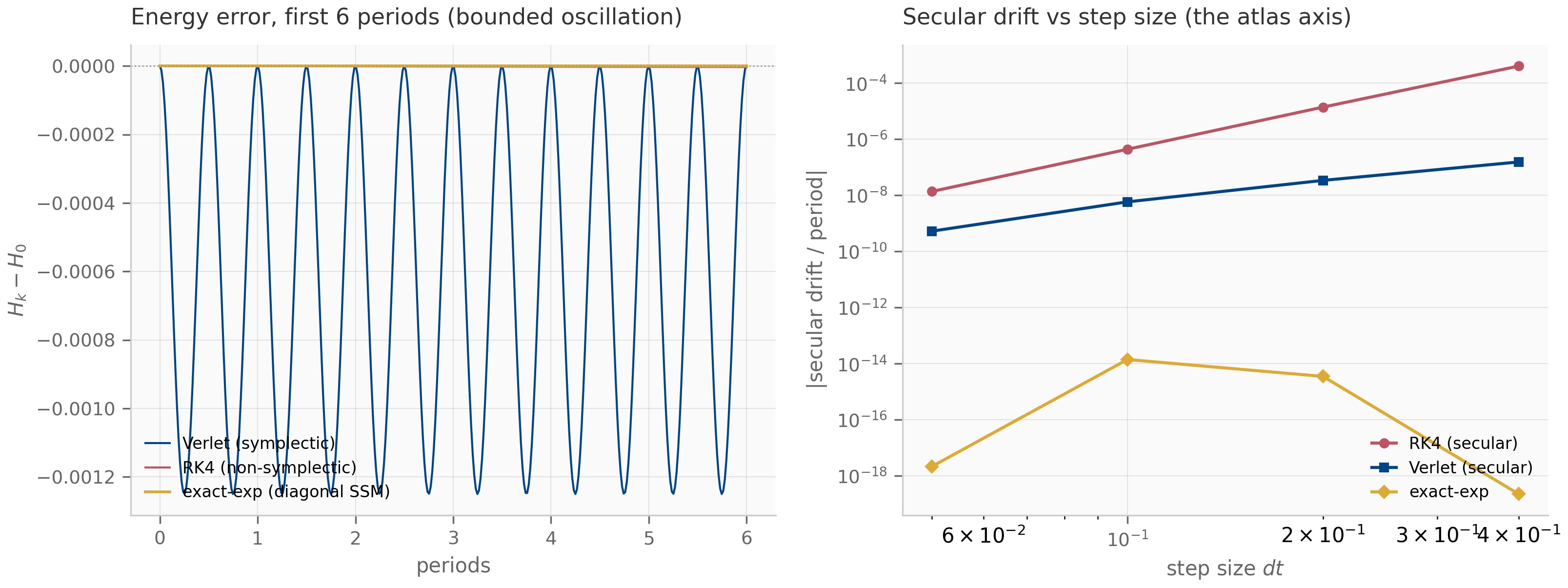
The reading is sharp, and it is the C1 pilot’s premise in miniature. A symplectic integrator (Verlet) buys zero secular energy drift at the cost of a larger bounded oscillation; a non-symplectic one (RK4) has a smaller oscillation but accumulates drift. But the diagonal SSM’s exact exponential dominates both — it has neither drift nor oscillation, because exponentiating a purely imaginary eigenvalue is exactly energy-preserving. The classical symplectic-versus-standard contest is moot for a diagonal SSM. This is not a null result for C1 — it sharpens the pilot’s target: the symplectic advantage can only reappear where the exponential is not applied exactly — a coupled or non-normal transition (the matrix memories of Proposition 13.1), or the forced integral handled at finite order. Whether a trained selective SSM drifts off the diagonal far enough for that to matter is exactly the empirical question the C1 pilot’s symplectic atlas pursues on real matrices — and which this idealized cell cannot answer, only frame. The pilot’s code and findings live in the predecessor repository’s C1 kickoff.
17.3 B — two-timescale benchmarks, and a disentanglement pipeline
The B pilot asks whether an architecture separates a fast process (token bigrams) from a slow one (regime drift). Chapter 14 built the two-timescale HMM and its matched-decay optimality (Theorem 14.4, Theorem 14.1); Chapter 16 built the probing protocol and the paired-comparison statistics (Proposition 16.1, Proposition 16.2); Chapter 15 built the diagnostics, including effective state size (Proposition 15.3). Each measured one facet. The integration runs all three end-to-end on the same reference instance and asks whether the facets cohere.
For each idealized predictor on the known HMM, the pipeline computes three numbers: the effective state size of its regime-propagation operator (Chapter 15, the participation ratio of the operator’s spectrum), its regime-recovery probe accuracy (Chapter 16, a held-out ridge probe of the true regime from the predictor’s carried state), and its predictive cross-entropy (Chapter 14).
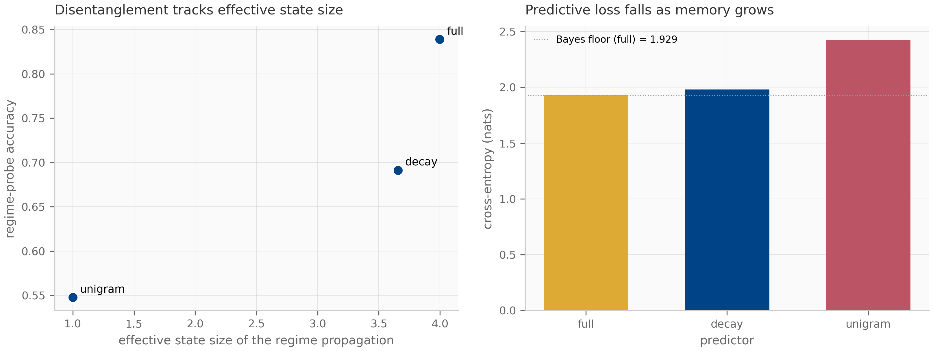
The three instruments cohere: a predictor’s effective state size, its disentanglement, and its loss move together. The comparison is made honest by Chapter 16’s paired statistics: the decay-versus-full per-token loss gap is a measured nats, with a paired standard error of against an unpaired — the shared per-token difficulty (correlation ) is subtracted off, resolving a gap that an unpaired comparison would call marginal. This is the protocol of Proposition 16.2 turned on the pilot’s own task.
Every predictor here is an exact idealization on a known HMM — there is no trained model and no fitted probe target beyond the closed-form filters. The pilot’s contribution is to run this same pipeline on trained checkpoints: probe a real layer’s regime recovery against its measured effective state size, and read its disentanglement against the impossibility ceiling (Proposition 15.1). That program — generators, baselines, the harness — lives in the B kickoff.
17.4 The 13-niche portfolio and the decision rubric
C1 and B are two cells of a larger catalog. The curriculum was designed against a 13-niche portfolio — research directions a numerical-analyst’s reading of sequence models opens up — grouped into four families. The table below maps each niche to representative chapters it draws on as shipped (the author’s reading of the finished book — not the design-time dependency matrix, which together with the full taxonomy and per-niche kickoffs lives in the predecessor’s curriculum design and niche decision).
| Family | Niche | One line | Draws on | Status | |---|---|---|---|---| | A (diagnostics) | A1 Discretization atlas | catalog integrators against SSMs and step sizes | Ch 4–6, 10 | portfolio | | | A2 Update-rules-as-integrators | delta-rule updates as ODE solvers | Ch 6, 12 | portfolio | | | A3 Diagnostics toolkit | Lyapunov spectra + effective state size on trained models | Ch 2, 15 | portfolio | | | A4 Multi-signal regime detection | combine signals to localize regime boundaries | Ch 9, 15 | portfolio | | | A5 Gather-and-Aggregate | the head-importance mechanism behind the recall gap | Ch 14, 15 | portfolio | | B (benchmarks) | B Two-timescale benchmarks | disentangle fast from slow; the §17.3 pipeline | Ch 12, 14, 15, 16 | active (parallel pilot) | | C (NA core) | C1 Symplectic integrators | structure-preserving discretization; the §17.2 atlas | Ch 1–3, 6, 10 | active (primary pilot) | | | C2 Stiffness analysis | is the stiff regime the real training issue? | Ch 5, 6 | portfolio | | | C3 Krylov / matrix-free | the SSD scan as a Krylov target | Ch 3, 9 | portfolio | | | C4 HiPPO conditioning | conditioning of the HiPPO construction | Ch 3, 7 | portfolio | | D (theory) | D1 Reachability | control-theoretic reachability of SSM states | Ch 1, 2 | portfolio | | | D2 Spectral biographies | eigenvalue trajectories across training | Ch 2, 13, 15 | portfolio | | | D3 ODE-solver-as-architecture | architectures named by their integrator | Ch 5, 6, 10 | portfolio |
The two active pilots were not chosen by enumerating value; they were chosen by a decision rubric worth stating, because it generalizes. (i) Direct-transfer depth — C1 is the same symplectic mathematics the author already knows, on a new object, not a loose analogy. (ii) A shared publishing window — A1, C1, and C2 all bear on the exp-trapezoidal integrator and share the Mamba-3 window, so picking any one keeps the family alive. (iii) Non-overlapping machinery — C1 (geometric integration) and B (singular perturbation) use disjoint tools, so they run in parallel without competing for the same hours. (iv) Paid-up-front cost and a documented-null fallback — C1 ships a structural-classification result even if its empirical case returns negative. The other eleven niches stay in the portfolio as documented alternatives, each with the chapters it would draw on already in hand.
17.5 What the lens earned, and its limits
So: did the dynamical-systems lens earn its keep? The honest answer is provisionally yes, and here is exactly how far the evidence reaches.
What it earned is the questions, posed precisely and instrumented. “Is exp-trapezoidal leaving Hamiltonian structure on the table?” is not a question the architecture literature asks; it is natural only once an SSM mode is a discretized ODE and the integrator is a choice with a conservation budget (§17.2). “Does effective state size govern disentanglement?” is measurable only once the state has a spectrum and a participation ratio (§17.3). The lens turned vague intuitions — “Mamba is unstable at long horizons”, “hybrids recall better” — into quantities with diagnostics: Lyapunov exponents (Proposition 15.2), effective state size, the probe signature.
What it has not earned, and cannot from this chapter, is an empirical verdict. Every number here is from an idealized system; the trained-model evidence is the pilots’ forthcoming work. And two limits bound even that future evidence. The first is the cited ceiling: the circuit-class impossibility ( Merrill et al. (2024) ; the book’s own counting bound, Proposition 15.1, is its weaker, architecture-agnostic shadow) means no amount of clever discretization or benchmarking lets a fixed-state recurrence do what the complexity class forbids — the pilots can measure where a model sits beneath the ceiling, never move it. The second is mechanistic: the Gather-and-Aggregate finding ( Bick et al. (2025) ) says the recall gap lives in a few attention heads, so a pure-SSM pilot result is read against a known mechanism, not in a vacuum. The lens is an instrument for locating a model in a landscape whose boundaries other tools drew; that is a real contribution, and a bounded one.
17.6 Where this goes
This is the last chapter, so “what’s next” is not more curriculum — it is the research the curriculum exists to enable. The two pilots execute on their own timelines: C1 builds the symplectic atlas on trained Mamba-3 matrices and negative-eigenvalue SSM extensions; B runs the §17.3 pipeline on trained hybrids and reports the disentanglement signature against the ceiling. Both are tracked in the predecessor repository, and both have a documented-null fallback so they produce an artifact either way. The other eleven niches wait in the portfolio with their prerequisites in hand.
With this chapter the book is content-complete: seventeen chapters from linear ODEs to a research program, every architecture read as a dynamical system. The remaining work is not authoring but upkeep — the ordinary maintenance of a living book, its open items tracked in the repository’s issues.
17.7 Exercises
Exercise 17.1 (short)
A constructed SSM mode has eigenvalue with small. Using §17.2, which integrator — exact-exponential, Verlet, or RK4 — best preserves the mode’s long-horizon energy decay rate, and why does the answer change if the mode is embedded in a coupled (non-diagonalizable) transition?
Solution
For the diagonal mode the exact exponential wins outright: its discrete transition is with magnitude , reproducing the true decay rate exactly at any step size, with no oscillation and no secular drift (the companion measures the conservative limit at a band of ). Verlet and RK4 only approximate and carry the oscillation/drift trade-off of §17.2. The answer changes for a coupled transition: when the state is not diagonalized (a non-normal matrix memory, Proposition 13.1), the exponential is not applied mode-by-mode and is no longer exact or cheap, and a structure-preserving integrator can beat a generic one — which is precisely the regime the C1 pilot tests on trained matrices.
Exercise 17.2 (short, code)
Run companions/ch17/jax/b_integration.py. Report the effective state size, probe accuracy, and
cross-entropy for the full / decay / unigram predictors, and the paired decay-vs-full standard error.
What does tell you here?
Solution
The readout is full , decay , unigram — probe accuracy and (negative) loss both monotone in effective state size. The paired comparison gives a mean gap nats with against . Because the two predictors are scored on the same tokens, their per-token losses are highly correlated (); pairing subtracts that shared difficulty (Proposition 16.2), so a gap that is only unpaired is paired. The lesson: report paired statistics when comparing predictors on a shared task, or you will under-resolve real differences.
Exercise 17.3 (short)
Pick a portfolio niche from §17.4 — say A3 (diagnostics toolkit) or D2 (spectral biographies). List the chapters it draws on and name the specific companion instruments you would compose to bootstrap it.
Solution
A3 (diagnostics toolkit) draws on Chapters 2 and 15: compose companions/ch15/jax/lyapunov_diagnostics.py
(lyapunov_spectrum, effective_state_size, the resolution-limit caveat) with Chapter 2’s
qr_lyapunov engine, and apply them to trained-model Jacobians. D2 (spectral biographies) draws on
Chapters 2, 13, and 15: track transition_spectrum (Chapter 13) and the effective state size across
training checkpoints, watching the eigenvalues’ trajectory — the §17.3 pipeline is the per-checkpoint
measurement, repeated over training. Both are the same move: take an idealized instrument validated
in the book and point it at trained data, the niche supplying the experimental design.
Exercise 17.4 (theory) — solution in §17.8
Make the §17.2 bridge precise. Show that the harmonic oscillator in the complex coordinate satisfies , that the exact discrete transition over a step has magnitude , and conclude that a diagonal SSM with a purely imaginary eigenvalue conserves the mode energy under the exact exponential. Then argue when a symplectic integrator is nonetheless needed.
Exercise 17.5 (theory) — solution in §17.8
Design a two-timescale evaluation for a given pair of architectures, respecting Chapter 16’s discipline: size the task to the discriminative regime (Proposition 16.1), use the distractor rule, and use paired statistics. State precisely what measured outcome would count as a resolved disentanglement difference between the two architectures, and why an unpaired comparison could miss it.
Exercise 17.6 (theory) — solution in §17.8
Argue from the capacity bound (Proposition 15.1) what the C1 and B pilots can and cannot hope to demonstrate. Specifically: can either pilot’s empirical win raise a fixed-state model’s expressive ceiling, or only locate the model beneath it? Frame the answer in terms of the cited-versus-demonstrated boundary of §17.1.
17.8 Full solutions to theory exercises
Solution to Exercise 17.4
Write . Then . Factor: , so exactly. The continuous solution is , and the exact discrete transition over a step is multiplication by , whose magnitude is . The mode energy is , and since , the energy is constant for all — conserved exactly, with no oscillation and no drift (the companion measures a band of , i.e. machine precision). A diagonal SSM applies mode-by-mode, so it inherits this exactness on every imaginary mode; the symplectic machinery of Chapter 6 buys nothing it does not already have. A symplectic integrator is needed only when the exponential is not applied exactly: a non-normal or coupled transition (where diagonalization is unavailable or ill-conditioned, Proposition 13.1), or the forced/input integral handled at finite order (Theorem 10.1), where a structure-preserving step can keep the conservation budget a generic step spends.
Solution to Exercise 17.5
Size the task so the load sits in the discriminative regime of Proposition 16.1: the two architectures must differ in the capacity the task probes, or the benchmark measures nothing about them (a knee-region requirement, the §16.2 lesson). Construct the separation with the distractor rule — pad with content (fresher competing writes), not neutral fillers, since neutral padding is provably inert under an argmax read-out. Score each architecture’s per-item predictive loss (or probe accuracy) on the same sampled sequences, and compute the paired statistics of Proposition 16.2. A resolved difference is one whose paired confidence interval excludes zero. An unpaired comparison can miss it because the per-sequence difficulty is shared (both architectures find the same sequences hard), inflating by the shared-difficulty variance that pairing removes — as in §17.3, where the same gap is marginal unpaired and decisive paired. One must also pre-register the suite and avoid post-hoc subset selection, or the selection inflation of Proposition 16.3 manufactures a difference.
Solution to Exercise 17.6
Neither pilot can raise the ceiling. The capacity bound (Proposition 15.1) and the cited impossibility ( Merrill et al. (2024) ) are statements about every fixed-state recurrence: they bound what such a model can compute regardless of how it is discretized (C1) or benchmarked (B). A better integrator changes the numerical fidelity of the discretization, not the model’s expressive class; a better benchmark changes what we can measure, not what the model can do. So a C1 empirical win means “a structure-preserving integrator tracks this trained mode’s dynamics with less drift”, and a B win means “this architecture’s effective state size lets it disentangle to this measured degree” — both locate the model beneath the ceiling, with higher resolution than before. That is exactly the cited-versus-demonstrated boundary of §17.1: the ceiling is cited (a theorem of others, about a complexity class), and the pilots demonstrate position beneath it (measurements, on trained models). Confusing the two — claiming an integrator or a benchmark “breaks” an impossibility result — is the error the boundary exists to prevent.
17.9 Companion code
The companions live in companions/ch17/{jax,julia} and are float64 throughout; they compose
shipped instruments rather than introduce new kernels, so there is no torch port (it would only
re-run the JAX modules). Each produces a new integrated signature; the component values reduce to the
originating chapters’ (pinned in the tests).
jax/c1_integration.py— the C1 atlas cell (§17.2). Composes Chapter 6’s symplectic/RK4 steppers and Chapter 10’s complex-mode recurrence to compare the long-horizon energy conservation of the exact-exponential, Verlet, and RK4 integrators on a harmonic-oscillator SSM mode. The reused RK4 path reproduces Chapter 6’srk4_drift_per_periodexactly. Producesc1-atlas-cell.png.jax/b_integration.py— the B disentanglement pipeline (§17.3). Composes Chapter 14’s HMM and idealized predictors, Chapter 16’s probe signature and paired comparison, and Chapter 15’s effective state size into one readout linking effective state size, probe accuracy, and loss across the predictor family. Producesb-disentanglement.png.julia/symplectic_crosscheck.jl— a stdlib-only, independent-language cross-check of the C1 atlas cell (the C1 pilot’s atlas is itself Julia), matching the JAX energy-conservation signatures to .
PYTHONPATH=. python companions/ch17/jax/c1_integration.py
PYTHONPATH=. python companions/ch17/jax/b_integration.py
make companion-jax-tests # all chapters' JAX suites
julia --project=companions/ch17/julia companions/ch17/julia/runtests.jl