HiPPO theory: orthogonal-basis projection operators

7.1 The online function-approximation problem

A recurrent model carries a finite state $\statevec_t \in \R^N$ and updates it one sample at a time. The central question is what should that state store? HiPPO’s answer is sharp: the state should store a compressed representation of the entire input history, chosen so that the history can be reconstructed as accurately as $N$ numbers allow.

Make this precise. Fix a time $t > 0$ and consider the input seen so far, $u(s)$ for $s \in [0, t]$. Equip the interval with a measure $\omega_t(s)$ (a weighting that says which parts of the history matter). The best $N$-term approximation of $u$ in the weighted space $L^2(\omega_t)$ is its orthogonal projection onto an $N$-dimensional subspace spanned by basis functions $g_0, \dots, g_{N-1}$:

The coefficient vector $c(t) = (c_0(t), \dots, c_{N-1}(t))^\top$ is the compressed memory. HiPPO’s discovery is that for well-chosen bases $c(t)$ obeys a linear ODE in $t$ — so maintaining the optimal projection online is exactly running a linear state-space model.

The picture to keep in mind is reconstruction. Drive a signal into the operator, read off $c(t)$ at the final time, and expand $\sum_n c_n g_n$: you recover the history, and the recovery sharpens as $N$ grow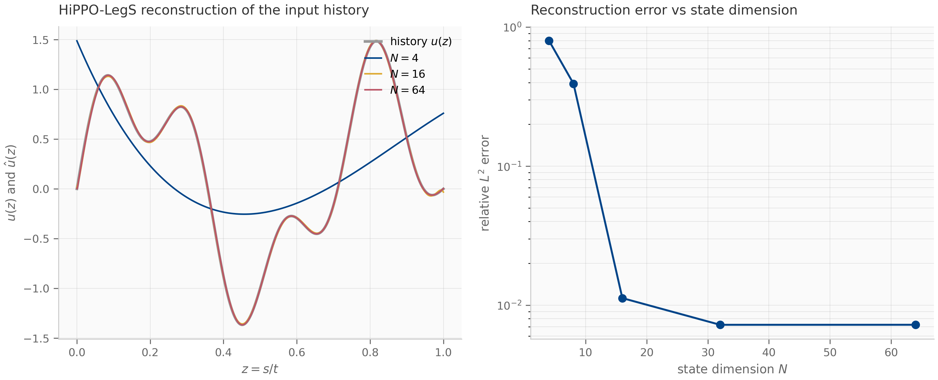s.

7.2 Orthogonal polynomial bases

The natural basis for functions on an interval is the Legendre polynomials $P_n$. On $[-1, 1]$ they are orthogonal under the uniform measure,

and satisfy the three-term recurrence $(n+1)P_{n+1}(x) = (2n+1)\,x\,P_n(x) - n\,P_{n-1}(x)$ with $P_0 = 1$, $P_1(x) = x$. Rescaling to the unit interval $z \in [0,1]$ and normalizing gives an orthonormal family

These are the basis functions HiPPO projects onto; the companion’s Gram-matrix check confirms their orthonormality to $10^{-3}$ under trapezoidal quadrature.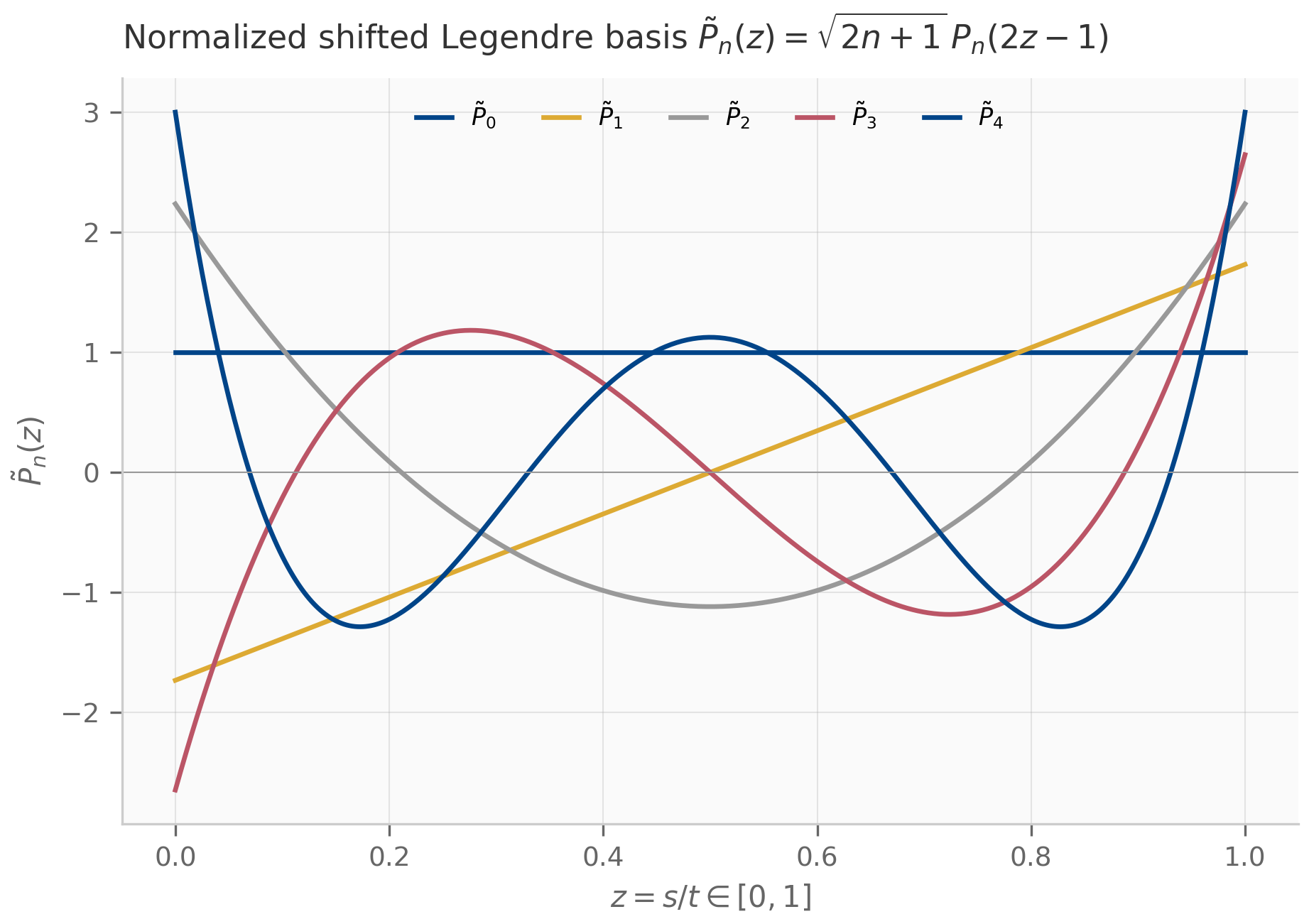

Orthogonality is what makes projection cheap and optimal. Because the basis is orthonormal, the best approximation is obtained coefficient-by-coefficient — no linear system to solve.

The proof (Exercise 7.5, §7.10) is the Hilbert-space Pythagorean theorem: the residual $u - \sum_n c_n g_n$ is orthogonal to $V$, so any other $v \in V$ only adds an orthogonal error that grows the norm.

The measure $\omega_t$ encodes which history matters. Two choices dominate the HiPPO literature Gu et al. (2020) :

• LegT (translated Legendre): a sliding window of fixed length $\theta$ — the state remembers the most recent $\theta$ time units uniformly and forgets everything older. This is a fixed-horizon memory.
• LegS (scaled Legendre): the growing window $[0,t]$ with uniform weight, rescaled as $t$ increases. The state remembers all history, allocating its $N$ coefficients to the whole past at every scale. This is the variant that gives S4 its long-range reach, and the one we develop in detail.

7.3 The HiPPO-LegS operator

For the scaled measure the projection coefficients obey a strikingly clean ODE. Differentiating $c_n(t) = \langle u, \tilde P_n\rangle$ through the time-dependence of the measure and using the Legendre recurrence yields the HiPPO-LegS dynamics, a linear state-space system whose matrices have a closed form.

The derivation (Exercise 7.4, §7.10) substitutes the Legendre three-term recurrence into the time-derivative of the projection integral; the lower-triangular structure is inherited from the recurrence, which expresses $P_{n+1}$ using only lower-degree polynomials. The matrix has a vivid signature: a negative diagonal that grows linearly, and negative off-diagonal entries below it that grow like $\sqrt{ij}$.

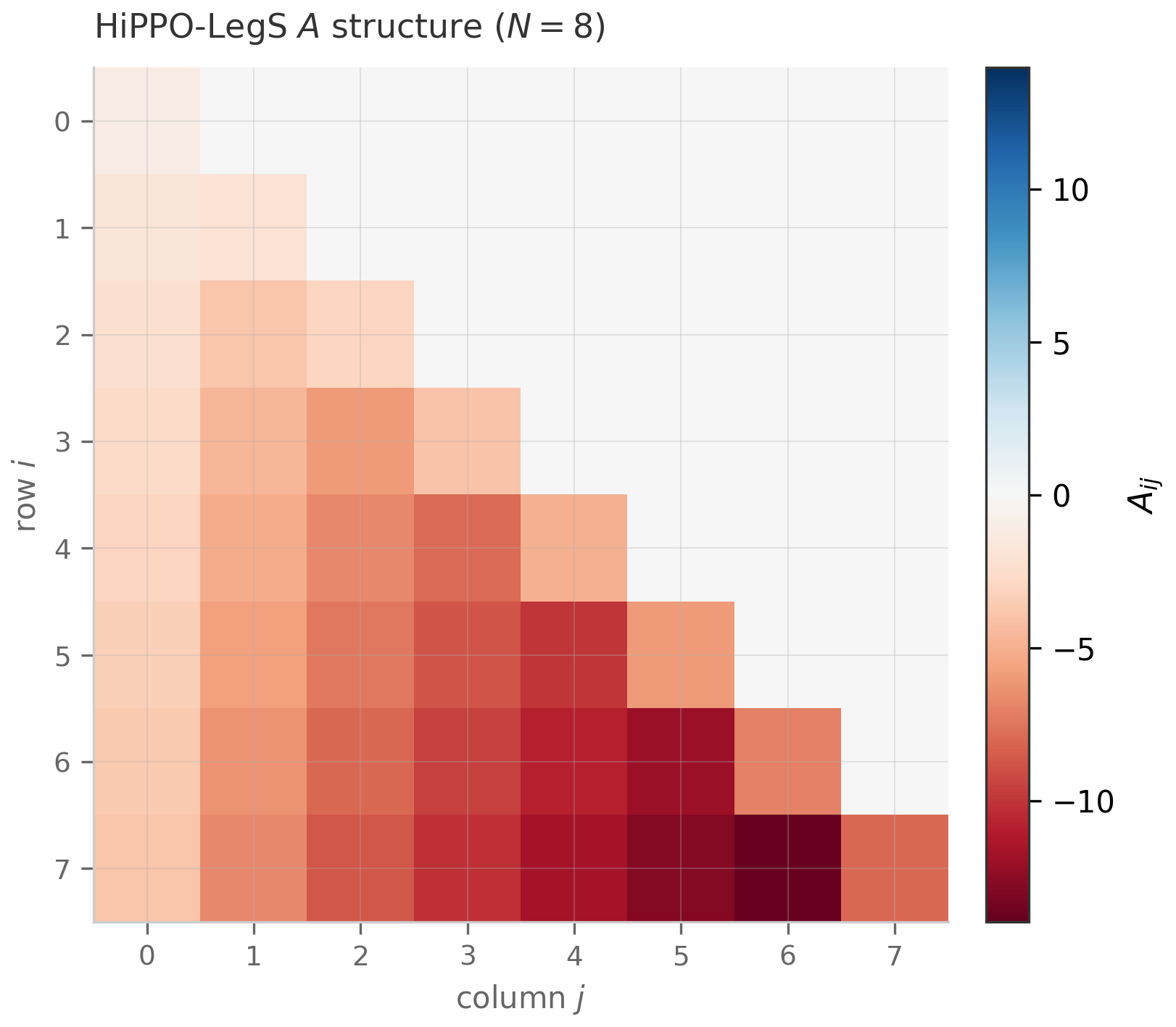
This is the answer to Chapter 4’s open question. Where Chapter 4 asked “given $\statemat$, how do we discretize it?”, HiPPO supplies the $\statemat$ — not by guessing, but as the projection-update operator of an optimal polynomial memory. Random initialization of $\statemat$ produces eigenvalues scattered across the complex plane and dynamics that vanish or explode over long horizons; the HiPPO $\statemat$ is engineered so that its discretization gives stable, long-memory recurrences Gu et al. (2020) .

7.4 From the operator to the S4-style recurrence

To run the HiPPO operator on sampled data we discretize the LTI system $\ddt \statevec = \statemat \statevec + \inputmat u$ exactly as in Chapter 4 §4.3. The zero-order hold gives

computed in practice through the augmented matrix-exponential trick of Chapter 4 (the HiPPO $\statemat$ is invertible — that promise from §4.3 is kept here). Because every eigenvalue of $\statemat$ has negative real part (§7.7), Chapter 4’s ZOH stability proposition applies verbatim: every discrete eigenvalue satisfies $\abs{\mu_i} = e^{\operatorname{Re}(\lambda_i)\stepsize} < 1$, so the recurrence is stable for any step size. ZOH is this book’s default discretization throughout Chapters 7–9 precisely because it preserves the HiPPO spectrum so cleanly (the original S4 paper used the bilinear transform instead, and S4D supports either; Chapter 4 §4.6 lays out the trade-off).

This recurrence is the recurrent view of an S4-style layer Gu et al. (2022) . Chapter 8 adds the second view — unrolling the recurrence into a convolution and computing it with an FFT — and shows the two views are identical for zero initial state. The HiPPO matrix is exactly the initialization that S4 places on $\statemat$ before training; S4D Gu et al. (2022) then diagonalizes it for speed, a move §7.5 explains is delicate precisely because of conditioning. Everything S4 does is downstream of the operator in §7.3.

7.5 Conditioning of the HiPPO basis

The HiPPO-LegS matrix is lower-triangular and its eigenvalues are the well-separated integers $-1, \dots, -N$ (§7.7), which sounds maximally benign. It is not, and the reason is non-normality: $\statemat$ is far from symmetric, so its eigenvectors are highly oblique and the matrix that diagonalizes it is ill-conditioned. The condition number of that eigenvector basis grows exponentially in $N$ Yu et al. (2023) , so a naive diagonalization of HiPPO-LegS is numerically untrustworthy at the $N$ used in practice — and the sub-quadratic conditioning one wants is achieved only by deliberately perturbing the transform (the “robustifying” construction below).

Two consequences follow. First, diagonalization is dangerous: S4D’s diagonal reparameterization Gu et al. (2022) must be done in a numerically careful (often complex, approximately-diagonal) form, and the “robustifying” line of work Yu et al. (2023) exists exactly to tame the conditioning of the diagonalizing transform. Second, the choice of discretization interacts with conditioning: a poorly conditioned basis amplifies the per-step error of a low-order scheme, so the second-order schemes of Chapter 4 (and the geometric integrators of Chapter 6) are not academic refinements but a response to a real failure mode. This conditioning question is the seed of research niche C4 — characterizing where HiPPO-style projections become numerically untrustworthy and what to do about it.

7.6 Alternative bases

Legendre is one choice among many; HiPPO is a framework parameterized by the basis–measure pair Gu et al. (2023) . Swapping the basis changes what the state is good at remembering:

• LagT (Laguerre): an exponentially-weighted infinite horizon — the measure decays into the past, so the state emphasizes recent history with a graceful tail.
• FouT (Fourier): a Fourier basis on a sliding window, well matched to periodic or oscillatory inputs; closely related to the implicit long convolutions of Chapter 11.
• Wavelet bases (WaLRUS): replacing polynomials with a redundant wavelet frame Babaei et al. (2025) shifts the optimal-projection target from polynomial smoothness to wavelet sparsity, which can suit signals with localized or multi-scale structure better than a global polynomial basis.

The “How to Train Your HiPPO” generalization Gu et al. (2023) derives the projection ODE for arbitrary measure–basis pairs and identifies which ones are well-conditioned to train — directly connecting basis choice back to §7.5. The lesson is that the structure of $\statemat$ (lower-triangular, stable spectrum, projection-update semantics) survives the basis change; the closed-form entries do not. When a later chapter reaches for a non-Legendre SSM, this is the machinery underneath.

7.7 Eigenvalue structure and stability

Return to the matrix itself. Because $\statemat$ is lower-triangular, its eigenvalues are exactly its diagonal entries.

The proof is immediate from lower-triangularity (Exercise 7.6, §7.10). The companion verifies it numerically: for $N$ up to $32$ the computed eigenvalues match $-1, \dots, -N$ to better than $10^{-8}$, and the strict upper triangle is exactly zero.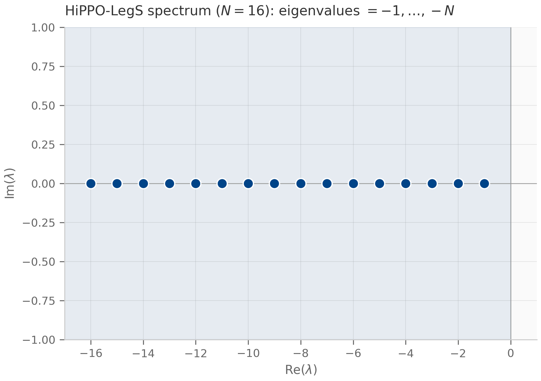

The integer spectrum has a memory interpretation: under ZOH the $n$-th mode decays per step by $e^{-(n+1)\stepsize}$, so low-index coefficients (coarse features of the history) are long-lived while high-index coefficients (fine detail) fade fastest. The state is a graded, multi-timescale memory — and the learnable $\stepsize$ slides the whole schedule. This is the dynamical-systems reading of why HiPPO works, and it is the structure a stability or Lyapunov analysis of a trained S4 layer (Chapter 15) measures against.

7.8 What’s next

This chapter answered “what is $\statemat$?” with “the projection-update operator of an optimal polynomial memory,” and showed that operator is lower-triangular, stably-spectrumed, and ZOH-discretizable into a recurrence. Chapter 8 takes that recurrence and develops the full S4 / S4D / S5 machinery: the convolutional view, the FFT kernel, the diagonalization that §7.5 warned is delicate, and the parallel scan. Chapter 9 then makes the parameters input-dependent — the selective SSMs (Mamba) — and Chapter 10 swaps ZOH for the exponential-trapezoidal scheme of Chapter 4 when the dynamics turn stiff. HiPPO is the hinge: every architecture from here inherits the structured $\statemat$ derived in §7.3.

7.9 Exercises

Six problems mixing computation and theory. Short/numerical (7.1–7.3) have inline collapsible solutions; the theory exercises (7.4–7.6) have full worked solutions in §7.10.

Exercise 7.1 (computation)

Using the three-term recurrence, write down $P_0, P_1, P_2, P_3$ and verify by direct integration that $\int_{-1}^{1} P_1(x) P_3(x)\, dx = 0$. Then confirm $\int_{-1}^1 P_2(x)^2\, dx = 2/5$.

Exercise 7.2 (computation)

Build the $4\times 4$ HiPPO-LegS matrix $\statemat$ from the closed form of §7.3 by hand. Verify that $\statemat_{31} = -\sqrt{21}$ and that the diagonal is $(-1, -2, -3, -4)$.

Exercise 7.3 (computation + code)

Run companions/ch07/jax/hippo_reconstruction.py. Confirm that the relative $L^2$ reconstruction error of the two-sinusoid test signal falls sharply from $N=4$ to $N=16$, then plateaus. Why does it plateau rather than continue to zero?

Exercise 7.4 (theory) — solution in §7.10

Show that the HiPPO-LegS matrix $\statemat$ is lower-triangular, and that its diagonal entries are $\statemat_{ii} = -(i+1)$, by appealing to the structure of the Legendre three-term recurrence. (You may take the off-diagonal closed form as given; the point is the structure.)

Exercise 7.5 (theory) — solution in §7.10

Prove the best-approximation theorem (Theorem, §7.2): if $\{g_n\}$ is orthonormal in $L^2(\omega)$ and $c_n = \langle u, g_n\rangle_\omega$, then $\sum_n c_n g_n$ is the unique minimizer of $\lVert u - v\rVert_\omega$ over $v \in \operatorname{span}\{g_n\}$.

Exercise 7.6 (theory) — solution in §7.10

Using lower-triangularity, prove that the eigenvalues of $\statemat$ are exactly $\{-1, \dots, -N\}$. Then show that ZOH discretization sends every eigenvalue strictly inside the unit disk for all $\stepsize > 0$, and identify the per-step decay rate of the $n$-th mode.

7.10 Full solutions to theory exercises

Solution to Exercise 7.4

The shifted Legendre polynomials satisfy a three-term recurrence in which $P_{n}$ is expressed through $P_{n-1}$ and $P_{n-2}$ — never through higher-degree polynomials. When the projection coefficient $c_n(t) = \langle u, \tilde P_n\rangle_{\omega_t}$ is differentiated in $t$, the time-derivative of the (scaled) measure couples $c_n$ to the inner products of $u$ against $\tilde P_m$ — and the recurrence guarantees only $m \le n$ appear. Hence $\ddt c_n$ depends on $c_0, \dots, c_n$ but not on $c_{n+1}, \dots$, which is exactly the statement that $\statemat$ has zero entries above the diagonal: $\statemat_{ij} = 0$ for $i < j$. For the diagonal, the “self-coupling” term of the $n$-th coefficient under the scaled measure contributes $-(n+1)$ (the normalization $\sqrt{2n+1}$ and the measure’s $1/t$ scaling combine to the integer $n+1$); this is the $\statemat_{ii} = -(i+1)$ claim. The off-diagonal entries $-\sqrt{(2i+1)(2j+1)}$ for $i>j$ follow from the same expansion carried through the normalization, given here without the full bookkeeping. $\blacksquare$

Solution to Exercise 7.5

Let $p = \sum_n c_n g_n$ with $c_n = \langle u, g_n\rangle_\omega$, and let $v = \sum_n a_n g_n$ be any element of $V = \operatorname{span}\{g_n\}$. First, the residual $u - p$ is orthogonal to every $g_m$:

using orthonormality $\langle g_n, g_m\rangle = \delta_{nm}$. Therefore $u - p \perp V$, and in particular $u - p \perp (p - v)$ since $p - v \in V$. Now decompose and apply the Pythagorean theorem:

with equality iff $\lVert p - v\rVert_\omega = 0$, i.e. $v = p$. So $p$ is the unique minimizer. $\blacksquare$

Solution to Exercise 7.6

A lower-triangular matrix has its eigenvalues on the diagonal: $\det(\statemat - \lambda I)$ is the product of diagonal entries $\prod_i (\statemat_{ii} - \lambda)$ because the determinant of a triangular matrix is the product of its diagonal, and subtracting $\lambda I$ keeps it triangular. With $\statemat_{ii} = -(i+1)$ the roots are $\lambda_i = -(i+1)$ for $i = 0,\dots,N-1$, i.e. exactly $\{-1, -2, \dots, -N\}$ — real, distinct, strictly negative.

Under ZOH the discrete dynamics matrix is $\discA = e^{\statemat\stepsize}$, whose eigenvalues are $\mu_i = e^{\lambda_i \stepsize}$. Then

so every discrete eigenvalue lies strictly inside the unit disk (A-stability, Chapter 4). The per-step decay rate of mode $n$ is $e^{-(n+1)\stepsize}$: higher-index modes decay faster, giving the graded multi-timescale memory of §7.7. $\blacksquare$

7.11 Companion code

Three runnable companions for Chapter 7 — the first SSM-core chapter, where the foundations and numerics threads meet in one operator. All three language tracks produce the same HiPPO-LegS matrix and the same reconstruction errors, which is itself the lesson: the mathematics is framework-independent; the idioms differ.

JAX (companions/ch07/jax/):

• hippo_matrix.py — builds the HiPPO-LegS $\statemat, \inputmat$ from the §7.3 closed form with a vectorized jnp.where (no Python loop, jit-fusable); emits hippo_matrix_structure.png and hippo_eigenvalues.png.
• hippo_reconstruction.py — runs the time-varying LegS recurrence via jax.lax.scan and reconstructs the history; emits legendre_basis.png and hippo_reconstruction.png.
• tests/test_hippo.py — pins the closed form, the integer spectrum, the reconstruction-error decay, and a lax.scan-vs-naive-loop equivalence guard.

Julia (companions/ch07/julia/):

• hippo_legendre.jl — the same operator with stdlib LinearAlgebra only; the encoder is an explicit for loop (the contrast to lax.scan), and the Legendre basis is built from the three-term recurrence.
• runtests.jl — @testset assertions including an orthonormality Gram-matrix check.

PyTorch (companions/ch07/torch/):

• hippo_operator.py — HiPPO-LegS wrapped as an nn.Module projection operator (fixed buffers, zero learnable parameters); a define-by-run eager loop encodes the signal. This is the object Chapter 8’s S4 layer extends.
• tests/test_hippo_torch.py — cross-framework consistency: the matrix matches the closed form and the reconstruction errors reproduce the JAX/Julia numbers.

To run from the repo root:

# JAX (uses the uv .venv with jax, numpy, scipy, matplotlib)
PYTHONPATH=. python companions/ch07/jax/hippo_matrix.py
PYTHONPATH=. python companions/ch07/jax/hippo_reconstruction.py

# Julia (stdlib only; instantiates instantly)
julia --project=companions/ch07/julia companions/ch07/julia/hippo_legendre.jl

# PyTorch (needs the .venv [torch] extra)
PYTHONPATH=. python companions/ch07/torch/hippo_operator.py

All figures emit to public/figures/ch07/.