Linear ODEs as state-space systems

1.1 What is a state-space system?

A linear state-space system is the pair of equations

where $\statevec(t) \in \R^N$ is the state at time $t \ge 0$, $u(t) \in \R^D$ is the input signal, $y(t) \in \R^M$ is the output, and the four matrices $(\statemat, \inputmat, \outputmat, \feedmat)$ are real-valued with shapes $N \times N$, $N \times D$, $M \times N$, $M \times D$. The first equation is the state equation — a first-order linear ODE describing how the state evolves. The second is the output equation — a static linear readout. The integer $N$ is the state dimension; it controls how much history the model can carry forward.

The pair is “linear” because both equations are linear in $\statevec$ and $u$ separately. It is “state-space” because $\statevec(t)$ summarizes everything the system needs from the past in order to predict the future given future inputs — a property called the Markov property of state. Given the present state and the input from now onward, the system’s entire future is determined.

A few conventions before going further. We treat $\statevec(t)$ as a column vector and apply $\statemat$ on the left: $\statemat \statevec$, not $\statevec \statemat$. We absorb the feedthrough term $\feedmat u(t)$ into the output equation only — it appears nowhere in the state dynamics — and we will often set $\feedmat = 0$ in examples to keep notation light. When the input is absent ($u \equiv 0$), the state equation reduces to

the homogeneous linear ODE, whose solution is the focus of §1.2.

Why this object

Three reasons the state-space form is the right starting point for a book on sequence-model architectures:

1. It separates dynamics from input. Whatever the input signal looks like, the dynamics matrix $\statemat$ alone determines the system’s long-run behavior — its stability, oscillation frequencies, and decay rates. Most of the analysis in Chapter 2 looks only at $\statemat$.
2. It generalizes immediately. Replacing the scalar derivative $\ddt$ with a finite difference yields a discrete recurrence (Chapter 4); replacing $\R$ with $\C$ admits oscillatory modes (Chapter 6, Chapter 10); replacing the constant $\statemat$ with an input-dependent $\statemat(u_t)$ yields the selective-SSM family (Chapter 9). Each generalization preserves the state-space skeleton.
3. It’s the form in which continuous-time models are discretized. Every SSM derivation in the literature starts from a continuous state equation and applies a numerical integration scheme to get a discrete recurrence. If you don’t know the continuous object, the discrete one is opaque.

1.2 The matrix exponential and fundamental solutions

The homogeneous ODE $\ddt \statevec = \statemat \statevec$ with initial condition $\statevec(0) = \statevec_0$ has a unique solution for every $\statevec_0 \in \R^N$ — and that solution is

where $e^{\statemat t}$ is the matrix exponential of $\statemat t$, defined by the same series as the scalar exponential:

The fundamental solution property — that $t \mapsto e^{\statemat t} \statevec_0$ solves the homogeneous ODE — is verified by differentiating the series term-by-term and using $\frac{d}{dt} \frac{(\statemat t)^k}{k!} = \frac{\statemat^k t^{k-1}}{(k-1)!}$. The resulting derivative is $\statemat \cdot e^{\statemat t} \statevec_0$, which matches $\statemat \statevec(t)$. Existence and uniqueness for the inhomogeneous case ($u \not\equiv 0$) follow the variation of parameters formula

an integral that recurs (in discretized form) as the convolution kernel of every LTI SSM in Chapter 8.

Eigenvalue structure determines everything

The matrix exponential’s behavior is governed entirely by the eigenvalues of $\statemat$. If $\statemat$ is diagonalizable, $\statemat = V \Lambda V^{-1}$ with $\Lambda = \diag(\lambda_1, \ldots, \lambda_N)$, then

So $e^{\statemat t}$ acts on the eigenbasis as independent scalar exponentials. The real parts of $\lambda_i$ control decay or growth: $\Re(\lambda_i) < 0$ means $e^{\lambda_i t} \to 0$; $\Re(\lambda_i) > 0$ means blow-up. The imaginary parts control oscillation frequency. Three regimes recur throughout the book:

1. All eigenvalues with negative real part — the system is asymptotically stable: every trajectory $\statevec(t) \to 0$ as $t \to \infty$. This is the regime in which a recurrence “forgets” its initial state, and it is the design target for the $\statemat$ matrices of S4, Mamba, and friends.
2. At least one eigenvalue with positive real part — the system is unstable: some initial conditions blow up. A trained SSM whose $\statemat$ drifts into this regime is the dominant numerical failure mode (Chapter 5).
3. Purely imaginary eigenvalues — the system is marginally stable and oscillates without decay. These are the energy-preserving modes of Hamiltonian systems and are the natural home of symplectic discretization (Chapter 6).

When $\statemat$ is not diagonalizable — when it has repeated eigenvalues with deficient eigenspaces — the matrix exponential picks up polynomial-in-$t$ factors on top of the $e^{\lambda_i t}$ terms. The Jordan normal form (Chapter 3, §3.1) gives the precise statement. In practice almost every $\statemat$ arising from random initialization or from physical systems is diagonalizable, and the polynomial-factor case shows up only at codimension-one boundaries in parameter space.

1.3 The damped harmonic oscillator

The canonical small example. A unit mass on a spring with stiffness $k > 0$ and damping coefficient $c > 0$, displacement $q(t)$, evolves according to Newton’s second law,

This is a second-order scalar ODE, not first-order, so it does not yet fit the state-space template. We lift it by treating velocity as an extra state coordinate: let $\statevec(t) = (q(t), \dot q(t))^\top \in \R^2$. Then $\ddt \statevec = \statemat \statevec$ with

This lifting trick — introduce auxiliary states to reduce ODE order to one — is the same procedure by which every higher-order ODE becomes a first-order state-space system, and it foreshadows how implicit higher-order schemes (Chapter 6) work internally.

The eigenvalues of $\statemat$ are the roots of the characteristic polynomial $\lambda^2 + c \lambda + k = 0$:

Three sub-cases follow from the sign of the discriminant $c^2 - 4k$:

• Overdamped ($c^2 > 4k$): two real negative eigenvalues. Both modes decay monotonically; the displacement approaches zero without oscillation.
• Critically damped ($c^2 = 4k$): a repeated negative eigenvalue $\lambda = -c/2$. The matrix $\statemat$ is in this case not diagonalizable, and the solution contains a $t \cdot e^{\lambda t}$ term.
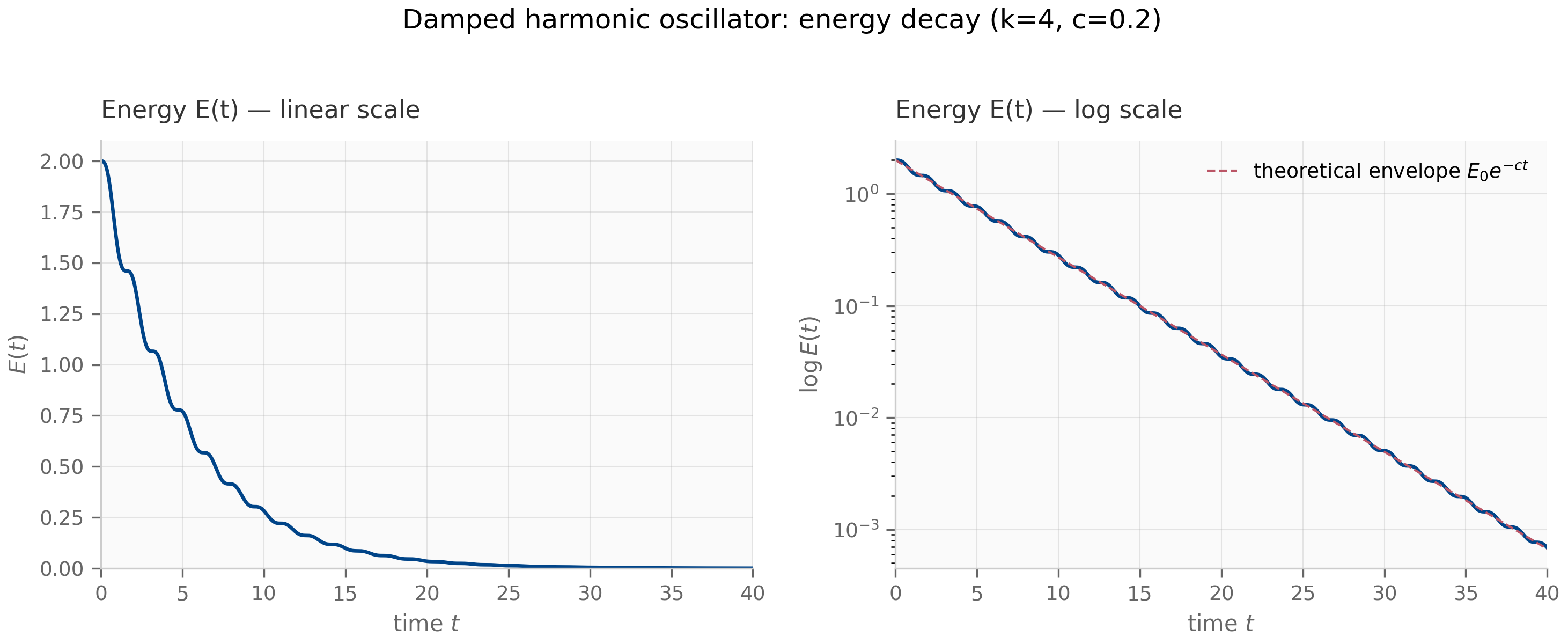
• Underdamped ($c^2 < 4k$): a complex-conjugate eigenpair $\lambda_\pm = -c/2 \pm i\omega$, with $\omega = \tfrac{1}{2}\sqrt{4k - c^2}$. Trajectories spiral toward the origin: oscillation at angular frequency $\omega$ with envelope decaying as $e^{-ct/2}$.

The total energy $E(t) = \tfrac{1}{2}(\dot q^2 + k q^2)$ is a useful diagnostic. Its time derivative is $\dot E = -c \dot q^2 \le 0$, i.e. energy decreases monotonically whenever $\dot q \ne 0$. Both stationary and oscillating trajectories satisfy this. The companion damped_oscillator.py simulates the underdamped regime and plots $E(t)$ alongside the trajectory; the energy curve gives an at-a-glance check that the numerical integration preserves the dissipation structure of the continuous system.

1.4 Coupled systems and the Jacobian

The damped oscillator is a 2-dimensional toy. Real systems — and trained SSMs — live in much higher dimensions, and they typically arise from coupling many simpler subsystems. The bookkeeping is straightforward once you accept that the state vector $\statevec$ stacks all subsystem states and $\statemat$ encodes both intra-subsystem dynamics and inter-subsystem coupling.

A useful larger example is a ring of coupled oscillators: $n$ identical damped oscillators arranged on a circle, each coupled to its two nearest neighbors by springs of stiffness $\kappa$. The displacements $q_1, \ldots, q_n$ and velocities $\dot q_1, \ldots, \dot q_n$ stack into a state vector $\statevec \in \R^{2n}$. The $\statemat$ matrix has a $2 \times 2$ block-diagonal structure for the per-oscillator dynamics, plus an off-diagonal coupling pattern that links each oscillator’s velocity equation to its neighbors’ positions:

with indices taken mod $n$. The bracketed term $q_{i-1} - 2 q_i + q_{i+1}$ is the discrete Laplacian of $q$ around the ring; it’s the same discretization of $\partial^2/\partial x^2$ you would use in a finite-difference method for the wave equation.

The $2n \times 2n$ Jacobian matrix $\jacobian$ — which for a linear system is just $\statemat$ — has eigenvalues that are easy to compute analytically because of the ring’s circulant structure. They come in complex-conjugate pairs

(for the underdamped regime). Each $m$ indexes a standing wave mode on the ring with wavenumber $2\pi m / n$; the $m=0$ mode is uniform translation (no spatial structure), $m = n/2$ (when $n$ is even) is the maximally-oscillating mode where adjacent oscillators move in antiphase. The companion coupled_oscillators.py constructs $\statemat$ for $n = 8$ and visualizes the eigenvalues in the complex plane.

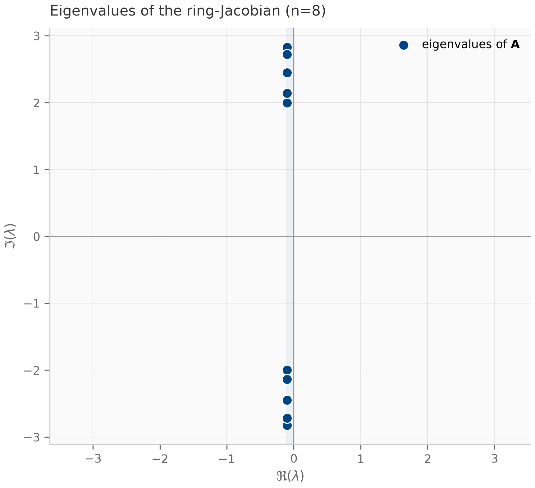
The key qualitative lesson: once you have the right state-space lift, even a system with rich spatial structure reduces to “compute eigenvalues of $\statemat$, classify by real and imaginary parts.” The eigenvalue distribution of a trained SSM’s $\statemat$ — pre-training, mid-training, and converged — is one of the most informative diagnostics you can compute (Chapter 2, §2.2; Chapter 5).

The Jacobian beyond linear systems

For a nonlinear system $\ddt \statevec = f(\statevec)$, the Jacobian $\jacobian(\statevec) = \partial f / \partial \statevec$ is the matrix of partial derivatives at $\statevec$. The linearization $\ddt \delta\statevec = \jacobian(\statevec^*) \delta\statevec$ around a fixed point $\statevec^*$ (where $f(\statevec^*) = 0$) describes how small perturbations $\delta\statevec$ evolve. The eigenvalues of $\jacobian(\statevec^*)$ then determine local stability of $\statevec^*$ by the same classification as in §1.2.

Trained recurrent networks — including SSMs in inference mode — are formally nonlinear (the state update is state = f(state, input) where f includes the input-dependent matrices). The linearization-around-a-state gives a local state-space system at each time step, and tracking how that local $\statemat$ varies along a trajectory is the foundation of the Lyapunov-exponent analysis in Chapter 2.

1.5 Phase portraits and the eigenvalue classification

A phase portrait is the geometric picture of all trajectories of an autonomous system in state space, drawn as oriented curves. For 2-dimensional linear systems $\ddt \statevec = \statemat \statevec$ on $\R^2$, the topology of the portrait is determined entirely by the trace $\tr(\statemat)$ and the determinant $\det(\statemat)$ — equivalently, by the eigenvalues — and the standard classification gives six qualitative behaviors:

The damped oscillator’s three sub-cases (over/critical/under-damped) realize three of these: stable node, stable degenerate node, stable spiral. The undamped limit $c \to 0$ slides the eigenvalues onto the imaginary axis, turning the spiral into a center; this is the Hamiltonian limit where energy is conserved exactly.

For higher-dimensional systems the topology is richer (think: 3-D systems can have spirals around line-shaped invariant manifolds), but the building blocks are the same: each pair of complex-conjugate eigenvalues contributes a 2-D spiral subspace, each real eigenvalue contributes a 1-D direction of decay or growth. This decomposition by invariant subspaces — equivalently, by the Jordan blocks of $\statemat$ — is the geometric content of the matrix exponential’s eigenvalue structure (§1.2).

1.6 A preview of frequency response

The variation-of-parameters formula

expresses the state as a convolution of the input with the kernel $K(t) := e^{\statemat t} \inputmat$. The output $y(t) = \outputmat \statevec(t)$ (taking $\feedmat = 0$) is therefore

The function $h(t) := \outputmat e^{\statemat t} \inputmat$ for $t \ge 0$ (and zero otherwise) is the impulse response of the system: the output you would observe if the input were a Dirac delta $u(t) = \delta(t)$.

Taking the Laplace transform turns convolution into multiplication. With $\widehat y(s) := \int_0^\infty y(t) e^{-st} dt$ and similarly for $\widehat u$, you get

where $H(s) := \outputmat (s I - \statemat)^{-1} \inputmat$ is the transfer function. The eigenvalues of $\statemat$ — already shown to govern $e^{\statemat t}$ — appear as the poles of $H(s)$, since $(sI - \statemat)^{-1}$ blows up exactly when $s$ equals an eigenvalue of $\statemat$. The poles’ location in the complex $s$-plane mirrors the eigenvalue classification of §1.5: left-half-plane poles ⇔ stable system; right-half-plane poles ⇔ unstable; imaginary-axis poles ⇔ marginally stable / oscillatory.

This connection is the bridge to Chapter 8, where you’ll see that the S4 layer’s convolutional view is literally a numerical evaluation of the impulse response $h(t)$ at uniformly spaced time points, and to Chapter 11, where the spectral structure of long convolution kernels (Hyena, RetNet) is analyzed via the same transfer-function framing.

1.7 What’s next

The next two chapters develop the analytical machinery that this chapter has only sketched. Chapter 2 makes the eigenvalue-stability story rigorous (Lyapunov, A-stability, BIBO) and adds the QR-based computational method for tracking eigenvalue trajectories during training. Chapter 3 introduces the structured-matrix vocabulary (Toeplitz, semiseparable, Vandermonde, Cauchy) needed to discuss the kernel constructions of S4 and friends. Chapters 4–6 then take the continuous state-space system here and discretize it — first crudely (ZOH, bilinear), then with full numerical-analysis machinery (Butcher tableau, A-stability), then via implicit and structure-preserving methods (Gauss–Legendre, symplectic integrators), which is where the active research pilot’s anchor (the C1 pilot) lives.

You can also profitably jump ahead: Chapter 8’s LTI SSM presentation reuses everything in this chapter and is self-contained for readers who want to see the SSM application before working through the full math foundation.

1.8 Exercises

Seven problems mixing computation and theory. Short/numerical exercises (1–4) have inline collapsible solutions; long/proof exercises (5–7) have full worked solutions in §1.9.

Exercise 1.1 (computation)

Compute the matrix exponential of $\statemat = \begin{pmatrix} 0 & 1 \\ -1 & 0 \end{pmatrix}$ by hand, term-by-term, and verify it equals the rotation matrix $R(t) = \begin{pmatrix} \cos t & \sin t \\ -\sin t & \cos t \end{pmatrix}$.

Exercise 1.2 (computation)

For the damped oscillator $\ddot q + c\dot q + k q = 0$ with $k = 1$ and $c = 0.5$, classify the damping regime and find the eigenvalues of $\statemat$.

Exercise 1.3 (computation)

Lift the third-order ODE $q''' + 2 q'' + q = u(t)$ into a 3-dimensional state-space system $\ddt \statevec = \statemat \statevec + \inputmat u$. Write $\statemat$ and $\inputmat$ explicitly.

Exercise 1.4 (computation)

For the ring of $n = 4$ identical damped oscillators with $k = 1$, $c = 0$, $\kappa = 0.5$ (no damping, symmetric coupling), use the formula in §1.4 to find the eigenvalues of $\statemat$ analytically. Confirm they lie on the imaginary axis (since $c = 0$) and verify by running companions/ch01/jax/coupled_oscillators.py with $n = 4$.

Exercise 1.5 (theory) — solution in §1.9

Prove that the matrix-exponential series $\sum_k M^k/k!$ converges absolutely (entrywise) for every square matrix $M$, with bound $\norm{e^M}_F \le e^{\norm{M}_F}$ where $\norm{\cdot}_F$ is the Frobenius norm.

Exercise 1.6 (theory) — solution in §1.9

Show that if $\statemat$ is skew-symmetric ($\statemat^\top = -\statemat$), then $e^{\statemat t}$ is orthogonal for every $t \in \R$ (that is, $(e^{\statemat t})^\top e^{\statemat t} = I$). Use this to give a geometric reason why the rotation matrix of Exercise 1.1 is orthogonal.

Exercise 1.7 (theory) — solution in §1.9

Prove the variation of parameters formula: the unique solution of $\ddt \statevec = \statemat \statevec + \inputmat u(t)$ with $\statevec(0) = \statevec_0$ is

1.9 Full solutions to theory exercises

Solution to Exercise 1.5

Let $\norm{\cdot}_F$ denote the Frobenius norm, which satisfies the sub-multiplicative property $\norm{AB}_F \le \norm{A}_F \norm{B}_F$. Then $\norm{M^k}_F \le \norm{M}_F^k$ by induction. Therefore

The partial sums are entrywise bounded by terms of a convergent scalar series, so each matrix entry is Cauchy in $K$ and converges. The limit is what we call $e^M$. The bound $\norm{e^M}_F \le e^{\norm{M}_F}$ follows by passing to the limit. ∎

Solution to Exercise 1.6

We have $\ddt e^{\statemat t} = \statemat e^{\statemat t}$ and $\ddt (e^{\statemat t})^\top = (e^{\statemat t})^\top \statemat^\top$. Let $Q(t) := (e^{\statemat t})^\top e^{\statemat t}$. Then

since $\statemat^\top + \statemat = 0$ by skew-symmetry. So $Q(t) = Q(0) = I$ for all $t$, i.e. $e^{\statemat t}$ is orthogonal.

Geometric interpretation: the rotation matrix $R(t)$ of Exercise 1.1 was generated by $\statemat = \begin{pmatrix} 0 & 1 \\ -1 & 0 \end{pmatrix}$, which is skew-symmetric. So $R(t)$ is orthogonal — which we already knew, but this derivation pins down why: orthogonality follows structurally from skew-symmetry of the generator, not from any property of the cos/sin functions. ∎

Solution to Exercise 1.7

Define $\statevec(t)$ by the formula on the right-hand side. We verify (a) the initial condition and (b) the ODE.

Initial condition. At $t = 0$ the integral vanishes (zero-length interval) and $e^{\statemat \cdot 0} = I$, so $\statevec(0) = \statevec_0$. ✓

ODE. Differentiate using the product rule on the integral (Leibniz’s rule for differentiating under the integral sign):

Uniqueness follows from the classical Picard–Lindelöf theorem applied to the right-hand side $f(\statevec, t) = \statemat \statevec + \inputmat u(t)$, which is Lipschitz in $\statevec$ uniformly in $t$ with constant $\norm{\statemat}$ (see Hairer–Nørsett–Wanner Hairer et al. (1993) for the standard proof). ∎

1.10 Companion code

Three runnable companions in companions/ch01/jax/:

• damped_oscillator.py — simulates the underdamped oscillator, plots energy decay (Figure 1.1)
• coupled_oscillators.py — constructs the ring-Laplacian state matrix, plots eigenvalue spectrum (Figure 1.2)
• matrix_exponential.py — compares scipy.linalg.expm against truncated series sums; the truncated series catastrophically diverges for matrices with large spectral radius (auxiliary, used by Exercise 1.5)

All companions import their plotting style from companions/_shared/plot_utils.py. To run from the repo root:

PYTHONPATH=. python companions/ch01/jax/damped_oscillator.py
PYTHONPATH=. python companions/ch01/jax/coupled_oscillators.py
PYTHONPATH=. python companions/ch01/jax/matrix_exponential.py

Figures are written to public/figures/ch01/ and referenced from the <Figure> components above.