Stability regions, Butcher tableau, and order conditions

5.1 Runge–Kutta methods and the Butcher tableau

Chapter 4 introduced ZOH, bilinear, and exp-trapezoidal as three specific one-step schemes for the linear state-space system. They are members of a much larger family: one-step methods that compute $\statevec_{k+1}$ from $\statevec_k$ using only one previous state and possibly intermediate stage evaluations of the right-hand side. The Runge–Kutta (RK) family is the most studied subfamily.

For the autonomous initial-value problem $\dot \statevec = f(\statevec)$ — we drop the explicit input dependence for this chapter; everything generalizes — an $s$-stage Runge–Kutta method computes

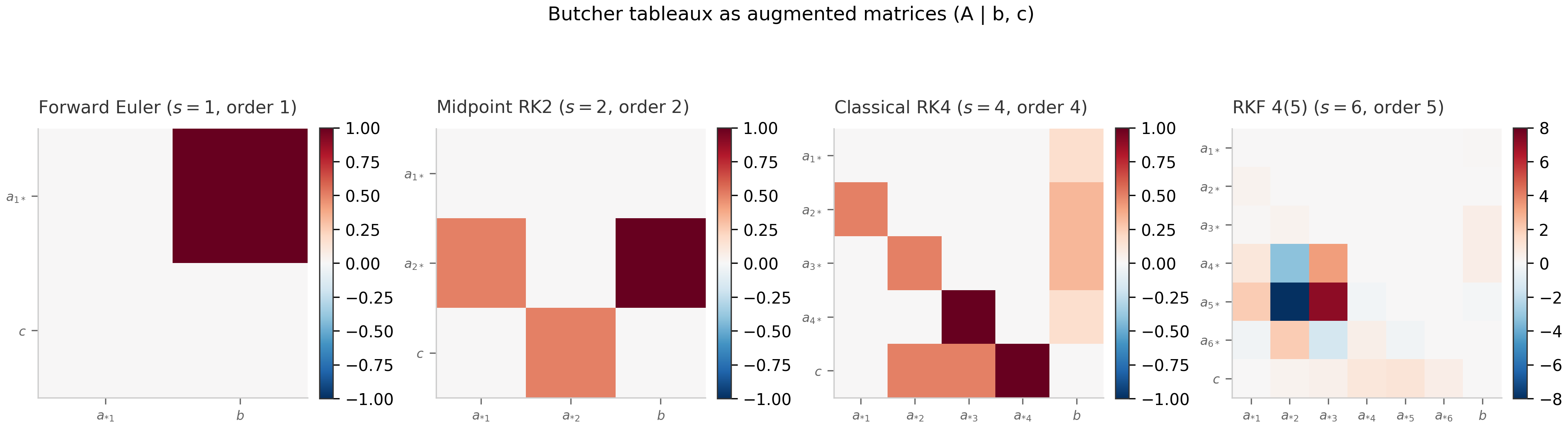
The $k_i$ are the stage derivatives — evaluations of $f$ at intermediate states. The constants $(a_{ij}, b_i, c_i)$ define the method, where $c_i := \sum_j a_{ij}$ are the stage times. The Butcher tableau is the standard tabular notation

The method is explicit if $A$ is strictly lower triangular ($a_{ij} = 0$ for $j \ge i$), in which case each $k_i$ depends only on previously computed $k_1, \ldots, k_{i-1}$. It is implicit otherwise, requiring a nonlinear system solve at each step.

Three classical examples make the formalism concrete.

Forward Euler. The simplest explicit method, $s = 1$:

The midpoint rule (RK2). A two-stage explicit method:

Classical RK4. The most-quoted explicit method, four stages:

Fourth-order globally, the workhorse of physics simulations for half a century.

The tableau abstraction was introduced by John Butcher in the 1960s and is now the lingua franca of one-step methods: every reference paper on numerical integration presents its method as a Butcher tableau. The constraint $\sum_j a_{ij} = c_i$ (consistency of stage times) and $\sum_i b_i = 1$ (consistency of the weighted sum) are imposed by every tableau worth its name. Without them the method does not even reproduce the trivial constant trajectory $\statevec(t) = \statevec_0$ when $f \equiv 0$.

5.2 Order conditions

How do we know that classical RK4 is fourth-order globally? The convergence order of an RK method is determined by order conditions: polynomial identities on the entries of $(A, b, c)$ that must hold for the local truncation error to be $O(\stepsize^{p+1})$.

The derivation expands $\statevec(t_k + \stepsize)$ as a Taylor series and matches term-by-term against the RK output $\statevec_{k+1}$ produced from $\statevec(t_k)$. For a scalar autonomous ODE the leading conditions are:

• Order 1: $\sum_i b_i = 1$
• Order 2: also $\sum_i b_i c_i = 1/2$
• Order 3: also $\sum_i b_i c_i^2 = 1/3$ and $\sum_{i,j} b_i a_{ij} c_j = 1/6$
• Order 4: four more conditions involving products of $b_i, c_i, a_{ij}$

For systems (the case we actually care about), the number of order conditions grows combinatorially: 5 conditions for order 4, 17 for order 5, 37 for order 6 Hairer et al. (1993) . Butcher organized these conditions using a bijection between order-conditions and rooted trees (each tree corresponds to an integer partition of $f$-evaluations and gives one polynomial identity). The combinatorial explosion is one reason 8th-order RK methods are rarely used: there are over 200 order conditions to satisfy simultaneously, and the resulting tableaux have dozens of stages.

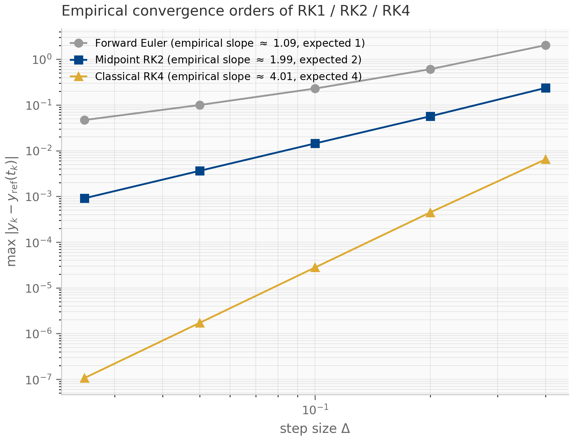
The proof is non-trivial and we will not reproduce it; the canonical reference is Hairer–Nørsett–Wanner Chapter II.2 Hairer et al. (1993) . For our purposes the takeaway is that the order of an RK method is a property of its tableau entries, derivable by algebraic manipulation alone. You can verify (Exercise 5.1) that RK4’s tableau satisfies all 4 order-4 conditions; you can also verify (Exercise 5.2) that an arbitrary two-stage explicit tableau cannot achieve order higher than 2, regardless of how you choose the free parameters.

5.3 The stability function and stability regions

Order conditions characterize how a method behaves as $\stepsize \to 0$ on a smooth problem. Stability characterizes how it behaves at fixed $\stepsize$ on a stiff problem — when the time scales in the dynamics are well-separated and at least one is much faster than $\stepsize$.

The standard probe is the Dahlquist test equation

The exact solution is $y(t) = e^{\lambda t}$. Applying an $s$-stage RK method to this scalar problem produces, after one step,

where $\stabfn : \C \to \C$ is the stability function of the method. For an explicit RK method, $\stabfn(z)$ is a polynomial in $z$ of degree $\le s$:

where $\mathbf{1}$ is the all-ones $s$-vector and the inverse expands as a finite geometric series because $A$ is nilpotent (strictly lower-triangular). For an implicit RK method, $\stabfn(z)$ is a rational function $P(z)/Q(z)$.

Three examples make this concrete.

Forward Euler. With $A = 0$, $b = 1$: $\stabfn(z) = 1 + z$.

Midpoint RK2. Working through the formula gives $\stabfn(z) = 1 + z + z^2/2$ — the second-order Taylor polynomial of $e^z$.

Classical RK4. $\stabfn(z) = 1 + z + z^2/2 + z^3/6 + z^4/24$ — the fourth-order Taylor polynomial.

A pattern emerges: for a $p$-th order explicit RK method, $\stabfn(z)$ agrees with $e^z$ through terms of degree $p$. This is no coincidence — order $p$ requires the method to reproduce $e^z$ correctly on the test problem through that order in $\stepsize$. The error $\stabfn(z) - e^z$ is $O(z^{p+1})$ near $z = 0$.

The stability region of the method is the set

On the test problem with $\lambda$ in the left half-plane (so the exact solution decays), the method’s iterates $y_k = \stabfn(\lambda \stepsize)^k$ stay bounded iff $\lambda \stepsize \in \stabregion$. The stability region is the constraint on $\lambda \stepsize$ that keeps the method well-behaved on stiff problems — equivalently, the set of $\stepsize$ values you can take for a given $\lambda$.

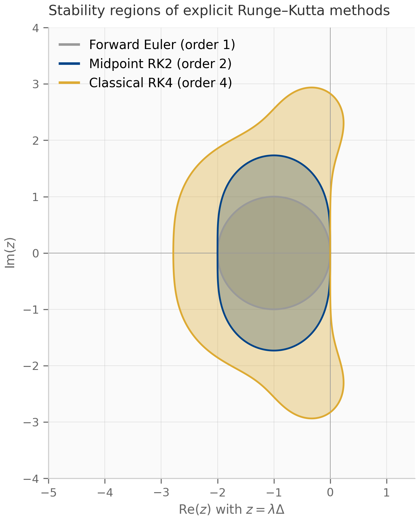
The stability region of forward Euler is the disk $\abs{1 + z} \le 1$ — a disk of radius 1 centered at $z = -1$. For a real-eigenvalue $\lambda < 0$, this requires $\stepsize \le 2/\abs{\lambda}$. The tighter this constraint becomes (large $\abs{\lambda}$ = stiff problem), the smaller the maximum step size — this is the step-size restriction that motivates implicit methods.

5.4 A-stability, L-stability, and the Dahlquist barrier

A method is A-stable if its stability region contains the entire closed left half-plane: $\stabregion \supseteq \set{z \in \C : \operatorname{Re}(z) \le 0}$. On a stable linear problem with $\operatorname{Re}(\lambda) \le 0$, an A-stable method preserves stability for every positive step size — no step-size restriction at all. This is the gold standard for stiff problems.

A method is L-stable if it is A-stable and $\stabfn(z) \to 0$ as $\operatorname{Re}(z) \to -\infty$. L-stability damps fast eigenmodes aggressively, which is desirable when you want the discrete method to not preserve fast oscillations the continuous solution decays. Backward Euler is L-stable; the trapezoidal rule (= bilinear from Chapter 4) is A-stable but not L-stable (its stability function $\stabfn(z) = (1 + z/2)/(1 - z/2)$ tends to $-1$, not 0, as $\operatorname{Re}(z) \to -\infty$). The distinction matters when the system has eigenvalues with very large negative real part: bilinear will preserve high-frequency oscillation modes that should physically be damped.

The fundamental theorem on A-stability of explicit methods is the Dahlquist barrier:

The proof for the explicit case is direct: an explicit RK method has $\stabfn(z) =$ polynomial in $z$, and any polynomial diverges as $\abs{z} \to \infty$. So $\stabregion$ is bounded, and cannot contain the entire (unbounded) left half-plane. ∎

The implicit case is more subtle: there exists an A-stable Runge–Kutta method of every order, but the constructions are increasingly elaborate. The Gauss–Legendre family — Chapter 6’s main attraction — produces A-stable implicit methods of every even order. The $s$-stage Gauss–Legendre method is order $2s$, optimally accurate among $s$-stage implicit RK methods, and A-stable, and (a bonus for Hamiltonian systems) symplectic.

The practical consequence for SSM discretization: you cannot have an explicit, A-stable, high-order one-step method. You must pick at most two of the three properties (explicit, A-stable, order ≥ 3). The Chapter 4 schemes resolve this trilemma differently:

• Forward Euler: explicit, order 1, not A-stable.
• ZOH and exp-trapezoidal: A-stable and of arbitrary order on autonomous problems, by virtue of using the matrix exponential — but they sit outside the explicit-RK family (they have non-polynomial stability functions).
• Bilinear: A-stable, order 2, implicit in form (requires inverting $I - \stepsize \statemat / 2$).

The exponential integrators of §4.5 are a way to evade the Dahlquist barrier: by computing $e^{\statemat \stepsize}$ exactly, the stability function inherits the full LHP-stability of the exponential, and the polynomial-order restriction is moved from $\stabfn$ to a different object (the approximation of the forcing by $\varphi$-functions). This is why exp-trapezoidal can be both “explicit in the input” (no nonlinear solve in $u$) and A-stable.

5.5 Stability regions of the Chapter 4 schemes

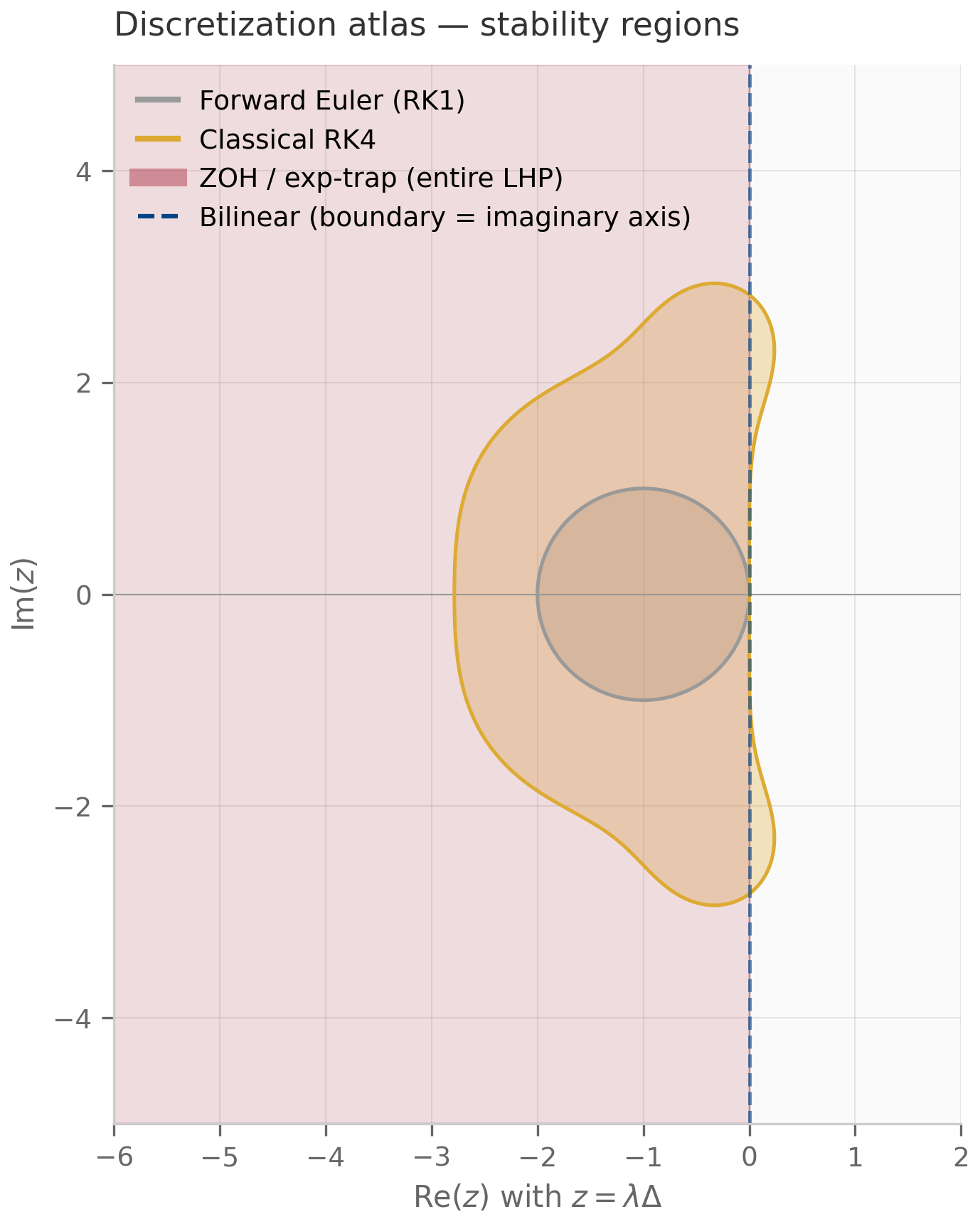
Reading the three Chapter 4 schemes through the lens of stability functions:

ZOH. From §4.3, $\discA = e^{\statemat \stepsize}$, so for the scalar test problem $\stabfn_{\text{ZOH}}(z) = e^z$. The stability region is $\set{z : \abs{e^z} \le 1} = \set{z : \operatorname{Re}(z) \le 0}$ — exactly the closed left half-plane. ZOH is A-stable, in fact also L-stable because $\abs{e^z} \to 0$ as $\operatorname{Re}(z) \to -\infty$.

Bilinear (Tustin). From §4.4, $\stabfn_{\text{bilinear}}(z) = (1 + z/2)/(1 - z/2)$. The Möbius geometry from Chapter 4 §4.4 / Exercise 4.5 says the LHP maps bijectively to the open unit disk, so the stability region is exactly the closed left half-plane — bilinear is A-stable. But $\stabfn_{\text{bilinear}}(z) \to -1$ as $\operatorname{Re}(z) \to -\infty$, so bilinear is not L-stable. This is the trapezoidal-rule failure mode: oscillatory artifacts on very stiff problems.

Exp-trapezoidal. The homogeneous stability function is identical to ZOH’s: $\stabfn(z) = e^z$ on the test problem (the difference between ZOH and exp-trap shows up only in the forcing integrals; the homogeneous behavior is the same). So exp-trapezoidal is A-stable and L-stable, just like ZOH.

5.6 What’s next

This chapter has laid out the systematic framework for analyzing one-step methods: Butcher tableau, order conditions, stability functions, stability regions, A-stability and L-stability, and the Dahlquist barrier. Chapter 6 uses this framework to motivate the implicit family — backward Euler, BDF, and the Gauss–Legendre IRK schemes that achieve A-stability at every order — and the symplectic family, which trades order or A-stability for the preservation of geometric invariants. Chapter 6 is where the C1 niche pilot lives: symplectic integration of selective SSMs viewed as Hamiltonian flows on the hidden-state manifold.

A natural side path is embedded methods — pairs of RK tableaux of consecutive orders sharing stages, used for adaptive step-size control. The DP54 method (Dormand–Prince 5(4)) used by DifferentialEquations.jl’s default solver Tsit5 is a famous example. Embedded methods are excellent practical tools but tangential to the SSM pedagogy of this book; the companion discretization_atlas.jl references the RKF45 / DP54 tableaux for completeness.

5.7 Exercises

Six problems. Short/numerical (5.1–5.3) have inline collapsible solutions; long/proof exercises (5.4–5.6) have full worked solutions in §5.8.

Exercise 5.1 (computation)

Verify that classical RK4 satisfies the four order-conditions of order 4 — at least the simpler ones: $\sum b_i = 1$, $\sum b_i c_i = 1/2$, $\sum b_i c_i^2 = 1/3$. Use the tableau in §5.1.

Exercise 5.2 (computation)

Show that an arbitrary two-stage explicit RK tableau (one free parameter $c_2 \in (0, 1]$, with $a_{21} = c_2$, $b_2$ to be determined, $b_1 = 1 - b_2$) cannot achieve order 3 no matter how $c_2, b_2$ are chosen.

Exercise 5.3 (computation + code)

Run companions/ch05/jax/order_verification.py. Confirm the empirical slopes match Forward Euler (1), midpoint RK2 (2), classical RK4 (4). What happens to the RK4 slope at very small $\stepsize$ (say $\stepsize = 10^{-4}$)?

Exercise 5.4 (theory) — solution in §5.8

Prove that for an explicit Runge–Kutta method with tableau $(A, b, c)$, the stability function is

where $\mathbf{1} = (1, 1, \ldots, 1)^\top$. Verify that for classical RK4 this evaluates to $1 + z + z^2/2 + z^3/6 + z^4/24$.

Exercise 5.5 (theory) — solution in §5.8

Prove the Dahlquist-barrier statement for explicit RK methods: that no explicit RK method is A-stable. (The proof was sketched in §5.4; flesh it out, using the fact that explicit methods have polynomial stability functions.)

Exercise 5.6 (theory) — solution in §5.8

For the bilinear/Tustin scheme, show that the stability function $\stabfn(z) = (1 + z/2)/(1 - z/2)$ satisfies $\stabfn(z) \to -1$ as $\operatorname{Re}(z) \to -\infty$ along any direction with $\operatorname{Im}(z)$ bounded, and explain why this rules out L-stability. Discuss what this means for the discrete dynamics of a bilinear-discretized stable LTI system with very fast-decaying eigenmodes.

5.8 Full solutions to theory exercises

Solution to Exercise 5.4

Apply the $s$-stage explicit RK method to the test ODE $\dot y = \lambda y$, $y(0) = y_k = 1$. The stage equations become

Set $z := \lambda \stepsize$ and let $\kappa = (k_1, k_2, \ldots, k_s)^\top$. The vector form is

For an explicit method $A$ is strictly lower-triangular, hence nilpotent ($A^s = 0$), and the geometric series $(I - z A)^{-1} = I + z A + z^2 A^2 + \cdots + z^{s-1} A^{s-1}$ truncates. So $\kappa = \lambda (I - z A)^{-1} \mathbf{1}$, and

For classical RK4, direct computation of $b^\top (I - z A)^{-1} \mathbf{1}$ — expanding the geometric series and multiplying out — gives, after some algebra,

This is the fourth-order Taylor polynomial of $e^z$, as expected for a fourth-order method.

Solution to Exercise 5.5

For an explicit RK method, $A$ is strictly lower-triangular, so $A^s = 0$ and the geometric series for $(I - z A)^{-1}$ truncates at $z^{s-1}$. Therefore

is a polynomial in $z$ of degree at most $s$. Polynomials are unbounded: $\abs{\stabfn(z)} \to \infty$ as $\abs{z} \to \infty$ along any ray (assuming the leading coefficient is nonzero, which holds for any $s$-stage method of order $\ge s$, the only interesting case).

The closed left half-plane $\set{z : \operatorname{Re}(z) \le 0}$ is unbounded — it extends to $-\infty$ along the real axis. The stability region \stabregion = \set{z : \abs{\stabfn(z)} \le 1} is therefore bounded. So $\stabregion$ cannot contain the entire LHP, and the method is not A-stable. ∎

The proof relies essentially on $\stabfn$ being a polynomial. Implicit methods have rational $\stabfn(z) = P(z)/Q(z)$, which can be bounded at infinity if $\deg(Q) \ge \deg(P)$. This is the precise sense in which implicit methods evade the Dahlquist barrier.

Solution to Exercise 5.6

Write $z = -r + i\omega$ with $r \to +\infty$ and $\omega$ bounded. Then

For large $r$ the dominant terms are $\stabfn(z) \approx (-r/2)/(r/2) = -1$. More precisely,

This rules out L-stability: L-stability requires $\stabfn \to 0$, not $\to -1$. ∎

Practical implication. For a stable LTI system $\dot \statevec = \statemat \statevec$ with $\statemat$ having an eigenvalue $\lambda$ with very large $\abs{\operatorname{Re}(\lambda)}$ — a fast-decaying mode — bilinear discretization at step size $\stepsize$ produces a discrete eigenvalue $\mu = (1 + \lambda \stepsize / 2)/(1 - \lambda \stepsize / 2) \approx -1$. The corresponding mode in the discrete dynamics therefore alternates sign at every step before decaying, rather than smoothly decaying. This trapezoidal-rule oscillation is the classic L-stability failure mode: the discrete solution exhibits spurious oscillations not present in the continuous solution. For SSMs this manifests as oscillatory artifacts in the hidden state when the system has eigenvalues with very negative real parts — exactly the regime where stiff implicit methods like BDF (Chapter 6) are preferred over bilinear.

5.9 Companion code

Two JAX companions and one Julia companion for Chapter 5.

JAX (companions/ch05/jax/):

• stability_regions.py — computes and plots stability regions for forward Euler, midpoint RK2, classical RK4, ZOH, bilinear, and exp-trapezoidal in the complex $z = \lambda \stepsize$ plane; emits rk_stability_regions.png, atlas_stability.png, and butcher_tableaux.png.
• order_verification.py — implements RK1/RK2/RK4 from their tableaux; verifies empirical orders 1, 2, 4 on the forced damped oscillator from Chapter 4; emits order_verification.png.

Julia (companions/ch05/julia/):

• butcher_tableau_zoo.jl — uses DifferentialEquations.jl solver tables (OrdinaryDiffEqTsit5, etc.) to extract Butcher coefficients programmatically and print them side-by-side with the analytic forms used in §5.1.
• Project.toml / Manifest.toml — companion-local Julia environment.

To run from the repo root:

# JAX
PYTHONPATH=. python companions/ch05/jax/stability_regions.py
PYTHONPATH=. python companions/ch05/jax/order_verification.py

# Julia (first run will precompile DifferentialEquations.jl)
julia --project=companions/ch05/julia companions/ch05/julia/butcher_tableau_zoo.jl

All figures emit to public/figures/ch05/.