Hybrid architectures and gating mechanisms

14.1 Two limits of sequence modeling

Part of this book’s argument has been that attention and state-space models are not rival species but two corners of one family. Chapter 9 made that literal: a selective SSM is a masked linear-attention computation (Theorem 9.5). Chapter 11 priced the recurrent corner: a finite additive state can hold only so many associations before interference swamps retrieval (Proposition 11.4), and Chapter 12’s delta-rule lineage bought back capacity with smarter writes at the cost of a genuine stability analysis (Theorem 12.4). The attention corner has the opposite ledger: retrieval is exact at any range it can see, and the price is a cache that grows linearly with what it has seen.

The trade is not hypothetical; it is the explicit organizing axis of the recall-throughput frontier mapped by Based Arora et al. (2024) : architectures that fix state size give up recall, architectures that keep recall give up the $O(1)$-per-token decode that makes long generation cheap. Pure designs sit at the frontier’s ends. The production systems of §14.5 sit deliberately in the middle, and the question this chapter equips you to ask is why the middle is the right place — not as an engineering compromise but as a statement about the sequences being modeled.

The statement is statistical. Real token streams mix two kinds of structure: fast, token-local dependence — syntax, local copying, the bigram-scale texture a short context pins down — and slow latent structure — topic, style, the document-level regime that changes rarely but conditions everything. (This decomposition-by-capability is also field practice: it is the premise of the synthetic-probe methodology of Poli et al. (2024) and Arora et al. (2024) that §14.6 takes up.) A layer that is exact over a short window serves the first; a compressed state that persists serves the second. Neither serves both: the window forgets the regime the moment it scrolls past the evidence, and the compressed state cannot reproduce exact local interactions it never stored. That intuition — two statistical timescales, two architectural resources — is the chapter’s lens. The next section gives it a theorem in the continuous prototype, and §14.6 an exactly computable discrete counterpart.

14.2 The two-timescale lens

The continuous prototype for “fast and slow living together” is a singularly perturbed linear system: a slow variable $x$ and a fast variable $y$ whose own dynamics relax on a timescale $\varepsilon \ll 1$,

with $D$ Hurwitz (every eigenvalue in the open left half-plane — a stable fast subsystem, the timescale separation that defines the stiff regime Chapter 6 tamed with implicit methods; Proposition 6.1). Setting $\varepsilon = 0$ formally gives $y = -D^{-1}C x$: the slow manifold, the surface on which the fast variable has equilibrated to whatever the slow variable is doing. What happens off the surface is the boundary layer: a transient, of duration $O(\varepsilon)$, in which $y$ collapses onto the manifold.

The proof is a change of variables and one Grönwall estimate. Differentiating $\eta$ along trajectories,

since $Cx + Dy = D(y + D^{-1}Cx) = D\eta$. The first term contracts at rate $\beta/\varepsilon$; the second is a bounded forcing of size $O(\varepsilon)$ on bounded trajectories. Variation of constants gives claim 1. For claim 2, substitute $y = -D^{-1}Cx + \eta$ into the slow equation: $\dot{x} = (A - BD^{-1}C)\,x + B\eta$, so the difference $e = x - x_r$ obeys $\dot{e} = (A - BD^{-1}C)\,e + B\eta$ with $e(0) = 0$, and Grönwall bounds $\|e(t)\|$ by a constant times $\int_0^t \|\eta\|$, which claim 1 bounds by $M\|\eta(0)\|\,\varepsilon/\beta + O(\varepsilon)\,T$. Exercise 14.4 carries the scalar case through explicitly; the nonlinear generalization is Tikhonov’s theorem Kokotović et al. (1986) .

The theorem licenses a reading of the hybrid division of labour — the reading Chapter 12’s closing section previewed:

• Attention is boundary-layer machinery. Within its window it computes pairwise interactions exactly — no compression, no model of how the past decays — which is precisely what fast, token-local structure needs, and exactly what a regime transient needs at the moment the slow context shifts.
• A decaying state is slow-manifold machinery. It carries a compressed, $O(1)$-size summary forward — the manifold parameterization — and its forgetting rate plays the role of the timescale assumption: Chapter 9’s selectivity and Chapter 11’s decay masks (Theorem 11.2) are mechanisms for making that rate fit the data’s slow rate.
• A hybrid is a matching construction. Sequential stacks, parallel gated blocks, and interleaved layers (§14.3) are different ways of joining the two descriptions — different matching conditions, in the asymptotics vocabulary.

What this lens does and does not claim. The theorem above is a statement about linear fast–slow ODEs, and in §14.6 an exact discrete counterpart is proved for a filtering task. The architectural reading — attention $\approx$ boundary layer, decaying state $\approx$ slow manifold, hybrid $\approx$ matched expansion — is an interpretive map between idealized computations, not a theorem about trained networks: nothing here claims that a trained hybrid implements a matching condition, and no such result exists. The map earns its keep where it is testable: it predicts which restriction fails on which statistics, and §14.6 measures exactly that. Its third leg is weaker, and we say so: the lens supplies the two specialists, not yet a theory of the joint — it does not by itself predict which matching condition (sequential, parallel, gated) wins where. The one careful cross-vendor comparison available — Lee et al.’s finding that sequential hybrids win at short context and parallel hybrids at long context Lee et al. (2025) — is consistent with components that specialize as the map says, and it is precisely the kind of data a theory of the joint would have to explain. Consistency is evidence for a lens, not proof of a mechanism; we will say “the lens predicts,” never “the network performs asymptotic matching.”

14.3 The composition design space

Fix the two primitives the rest of the chapter mixes, in the exact form the companion implements: sliding-window attention — causal softmax attention in which position $t$ attends to positions $t-w+1, \dots, t$ — and a gated-decay SSM, the per-channel EMA recurrence

the diagonal skeleton of Chapter 11’s gated linear attention, kept minimal so that every composition claim below is checkable to machine precision. Three composition patterns cover the production space:

1. Sequential: one primitive feeds the other within a block, $\mathrm{attn}(\mathrm{ssm}(x))$ or $\mathrm{ssm}(\mathrm{attn}(x))$ — the in-series pairing every stacked hybrid uses locally.
2. Parallel-gated: both read the same input and a gate blends them, $g \odot \mathrm{attn}(x) + (1-g) \odot \mathrm{ssm}(x)$ — the Hymba Dong et al. (2024) /GMU-style pattern, and the carrier of §14.4’s granularity question.
3. Interleaved at ratio $r\!:\!1$: a residual stack in which every $(r{+}1)$-th block is attention and the rest are SSM — the layer-ratio pattern, the design variable Chapter 12 deferred here from Kimi Linear’s 3:1 choice Kimi Team (2025) .

One boundary needs drawing, because the literature cuts this space twice. Sequential here is a within-block statement (primitives composed directly, no residual between them); a repeating block pattern — Griffin’s two recurrent blocks then one local-attention block, Jamba’s one attention block per eight — is an interleave in this vocabulary, whatever its authors call it. Lee et al.’s sequential-vs-parallel dichotomy Lee et al. (2025) is the coarser cut: their “sequential” covers every design in which information passes through the primitives in series — all interleaves included — against parallel-branch designs. We keep the finer three-way split and map their finding onto it where it is used (§14.5).

The companion pins the algebra that makes these well-posed objects of study (measured printouts; the tests pin each identity below $10^{-12}$): the band-masked windowed attention equals its per-position oracle to $4.4 \times 10^{-16}$; window $w \ge \seqlen$ is full causal attention (identical outputs, exactly); under constant input $\bar{x}$ the EMA matches its closed form $h_t = (1 - g^t)\bar{x}$ to $8.9 \times 10^{-16}$; and the parallel gate’s endpoint reductions are exact — $g = 1$ returns the attention branch bitwise, $g = 0$ the SSM branch.

Why does the ratio — rather than, say, the window alone — carry so much design weight? Because decode-time memory is the binding constraint at production context lengths, and the ratio sets it:

The proof is counting: each attention block holds a rolling $w \times d$ key buffer and a $w \times d$ value buffer; each SSM block holds its $d$-float state. The companion refuses to leave it at arithmetic — it materializes the buffers and asserts the formula against their actual sizes. At a production-shaped configuration ($n = 24$, $d = w = 1024$), the measured totals are $12{,}601{,}344$ floats at ratio $3\!:\!1$ and $6{,}312{,}960$ at $7\!:\!1$, against $3{,}221{,}225{,}472$ for full attention at $\seqlen = 65{,}536$ — factors of $255.6$ and $510.3$.

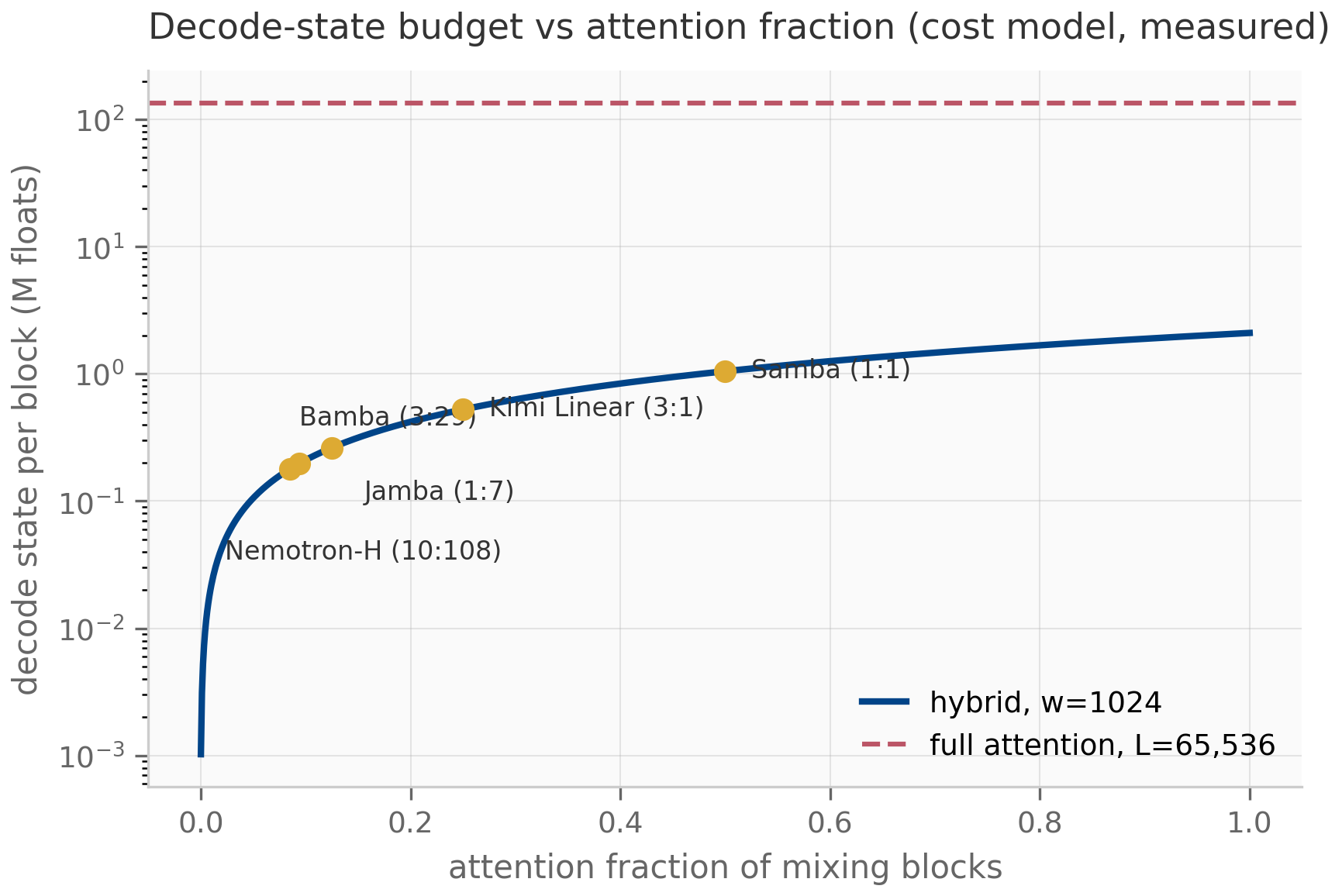
Two structural notes close the composition story. First, interleaving is the pattern that preserves trainability: every layer in the stack remains chunkwise-parallelizable — the SSM blocks by Chapter 11’s recurrent↔parallel duality and the delta-rule blocks by the WY machinery of Theorem 12.5 — so the ratio is a pure budget dial, not a training-throughput sacrifice. Second, the window and the ratio are not interchangeable: $w$ buys reach for the exact path, $f$ buys how often the exact path appears in depth. The two-timescale lens says their jobs differ in kind — $w$ must cover the fast structure’s correlation length, while the slow signal needs some carried state at some depth — and §14.6 measures exactly that asymmetry.

14.4 The gating design space

Composition decides where the two paths sit; gating decides, position by position and channel by channel, how much each path contributes. The production designs of §14.5 differ more in their gates than in anything else, and the differences organize cleanly along two axes.

Granularity — what shape the gate is:

The first strictness is a two-line argument: a $\{0,1\}$ vector gate that sends channel $1$ to attention and channel $2$ to the SSM would force a scalar gate to satisfy $g = 1$ and $g = 0$ simultaneously wherever the branches disagree on both channels. The second — input-dependent gates are genuinely stronger than constant ones — needs its two-input condition (a constant vector gate can already realize any single-input behaviour) and is Exercise 14.6. Both conditions hold generically for the actual attention/EMA branches. The companion pins the reductions and the channel-routing witness exactly (differences of $0.0$, not merely small). The lineup also uses one coarser point on the same axis: block granularity, where the “gate” is the structural choice of which block type occupies which position — a $\{0,1\}$ routing decision made once, at design time, for a whole block.

The ordering is the cheap part; the design question is where on it to sit. A scalar gate costs one number and one design meeting; a vector gate is Chapter 11’s decay-mask vocabulary (Theorem 11.2) applied to branch mixing; input-conditioned vector gates are exactly the move selective SSMs made in Chapter 9, now steering the blend rather than the state. Production examples, as of May 2026: Nemotron-H mixes with a fixed schedule and no per-channel gate NVIDIA (2025) . Gated DeltaNet’s decay gate is the scalar $\gamma_t$ per head Yang et al. (2025) — input-dependent but coarse — and Kimi’s KDA is precisely the per-channel (vector) refinement of it Kimi Team (2025) , the granularity class Griffin’s RG-LRU also occupies De et al. (2024) . SambaY’s Gated Memory Unit is an element-wise (vector) gate whose value is computed from a shared memory stream — input-dependent — while its placement across decoder layers is a fixed structural choice Ren et al. (2025) ; the trigger axis below classifies the value, not the wiring.

Trigger — what the gate responds to. A gate can be set by position (a fixed schedule: every $(r{+}1)$-th block, Hunyuan TurboS’s macro-block patterns Tencent Hunyuan Team (2025) ), by the input (every selective/gated recurrence above), or — the 2026 frontier — by the model’s own output state: AMOR invokes attention only at positions where prediction entropy crosses a threshold, reporting attention on roughly 22% of tokens with long-context stability Zheng & Shani (2026) . The trigger axis has a sharp theoretical caution attached: Basu’s analysis of content-based routing argues that mechanisms which avoid pairwise token comparison cannot route precisely (1–29% routing accuracy across recurrent, memory-bank, and bandit-style gates) — high-precision routing needs pairwise machinery, the representational ingredient cheap gates omit, though not necessarily full attention: the same paper constructs a 99.7%-accurate router from a rank-one pairwise projection at linear cost Basu (2026) .

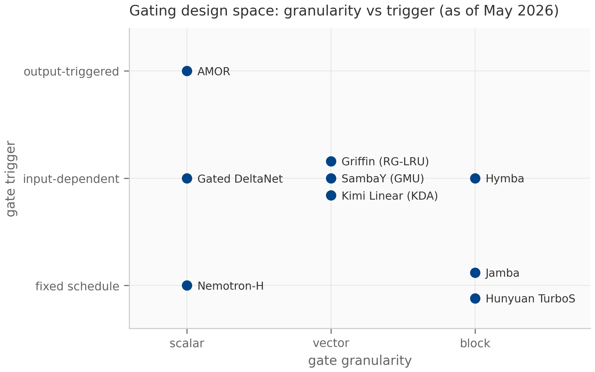
Two families that belong to this design space by shape are treated elsewhere: xLSTM’s exponential gates (granularity: vector; trigger: input; plus a stabilizer state the sigmoid families do not need) and the test-time memory writes of the Titans line (trigger: the loss, a fourth trigger class) are Chapter 13’s subjects, where their matrix-memory context lives.

14.5 The production lineup, as of May 2026

The lens and the design space were built to read a real lineup, so here it is.

| Model | Mix pattern (attention fraction $f$) | Gating | Reported headline (paper’s own) | |---|---|---|---| | Griffin De et al. (2024) | interleaved, 2 RG-LRU : 1 local attention ($f = 1/3$) | vector, input-dep. | matches Llama-2 quality with faster long-sequence inference | | Samba Ren et al. (2024) | interleaved 1:1 Mamba + sliding window ($f = 1/2$) | vector (Mamba’s) | linear-time training at 4K, length extrapolation to 256K context | | Jamba Lieber et al. (2024) | interleaved 1:7 attention:Mamba, MoE FFNs ($f = 1/8$) | block-structural | 256K context at 12B-active scale | | Bamba (IBM, HF blog) Bamba Team (IBM, Princeton, CMU, UIUC) (2024) | interleaved 3:29 attention:Mamba-2 ($f \approx 0.09$) | block-structural | fully open data recipe; ~2.5× vLLM decode throughput vs comparable transformers | | Nemotron-H NVIDIA (2025) | interleaved, 10 attention of 118 layers ($f \approx 0.08$) | scalar schedule | ~3× faster inference than similarly sized transformers at comparable accuracy | | SambaY / Phi-4-mini-flash Ren et al. (2025) | Samba self-decoder + GMU cross-decoder, single full-attention layer | vector (GMU) | ~10× decoding throughput on long-generation reasoning | | Hunyuan TurboS Tencent Hunyuan Team (2025) | AMF/MF macro-blocks (attention–Mamba–FFN), MoE | block schedule | top-10 LMSYS arena placement at 56B activated | | Kimi Linear Kimi Team (2025) | interleaved 3:1 KDA:full attention (MLA) ($f = 1/4$) | vector, input-dep. | 75% KV-cache reduction, up to ~6× decode at 1M context |

Read the table against Proposition 14.2 and the figure that draws it: every row sits low on the attention-fraction curve, exactly where the budget argument says the cheap exactness should be spent. The within-family motion is also informative: Samba → SambaY replaces cross-attention with a gate (GMU) and gains its throughput from the gating design space, not from a new mixing pattern; Jamba → Bamba → Nemotron-H is a march down the attention fraction as the slow-path layers improved (Mamba-1 → Mamba-2 Dao & Gu (2024) ); Kimi reaches the same neighbourhood from the delta-rule side, with Chapter 12’s gated-delta machinery as the slow path.

One cross-vendor regularity deserves its own sentence. Lee et al., comparing sequential against parallel mixing across vendors and scales, find sequential hybrids stronger at short context and parallel hybrids stronger at long context Lee et al. (2025) — the single most design-relevant empirical fact in the lineup. (Their dichotomy is the coarser cut §14.3 reconciled: “sequential” there spans the interleaves above.) Per §14.2’s flag, it is a consistency check for the matching lens — the kind of regularity a theory of the joint would have to explain — not a verification of it.

14.6 MAD and the two-timescale benchmark seed

How should claims like the table’s be tested? Full-scale training runs answer with averages over everything at once. The mechanistic-architecture- design (MAD) methodology Poli et al. (2024) answers with small, synthetic, capability-isolating tasks — in-context recall, compression, copying — chosen so that performance on the probe predicts scaling behaviour of the full architecture; the MQAR family Arora et al. (2024) did the same for associative recall specifically, and Chapter 11 already used it to measure the capacity wall. This section contributes the probe the two-timescale lens calls for, and it is pilot B’s seed.

The task. A hidden Markov model with the two timescales built in:

• a slow regime $z_t \in \{1, \dots, K\}$ with sticky transition $T(\varepsilon) = (1-\varepsilon)\,I + \tfrac{\varepsilon}{K-1}(J - I)$ — stay with probability $1 - \varepsilon$, else jump uniformly ($J$ the all-ones matrix);
• a fast process: given the regime, tokens follow a regime-specific bigram table, $P(x_{t+1} \mid z_{t+1} = j, x_t) = B_j[x_t, \cdot]$ on a vocabulary of size $V$;
• an overlap dial $\eta \in (0,1]$: the tables interpolate between a shared table and regime-specific ones, $B_j = (1-\eta)C + \eta D_j$, controlling how hard the regimes are to tell apart locally — measured by the mean per-token discrimination $\bar{\imath}$ (the average pairwise KL between regime rows).

Because the model is known, every predictor below is exact — no training, no approximation other than the stated information restriction — so every claim is a computation, checkable to machine precision. The Bayes-optimal predictor is the HMM forward filter, and the companion validates it against a brute-force enumeration over every regime path — $K^{t+1}$ paths for the prediction at position $t$, an independent code path that is only feasible on short validation instances ($\seqlen = 7$): maximum prediction difference $1.1 \times 10^{-16}$.

Three restrictions mirror the architectural resources:

• window-$w$ (the attention idealization): the same Bayes computation, restricted to the last $w$ tokens with a uniform regime prior at the window edge — exact pairwise machinery, zero carried state. With $w \ge \seqlen$ it reproduces the full filter exactly (difference $0.0$).
• fixed-decay (the state idealization): the filter run with the mixing-to-uniform prior update $M(\lambda) = (1-\lambda)I + \tfrac{\lambda}{K}J$ — a compressed state forgotten toward uniform at a fixed rate, the EMA of §14.3 wearing filtering clothes.
• unigram (the slow-manifold-only idealization): regime tracking with each bigram row replaced by the regime’s stationary unigram — carried state, no fast structure.

The fixed-decay restriction is the one with a theorem in it:

The proof is two lines of algebra on the diagonal and off-diagonal entries (Exercise 14.5). The companion measures the identity at $1.1 \times 10^{-16}$ entrywise and the resulting prediction agreement between the matched-decay filter and the optimal filter at $3.3 \times 10^{-16}$. This is the chapter’s sharpest statement of the slow-manifold half of the lens: gating is timescale matching. Chapter 9’s selectivity and Chapter 11’s decay masks let a model learn $\lambda$; the theorem says what the target of that learning is, and the V-shaped mistiming cost below says what missing it costs.

What each restriction costs, measured. At the committed reference configuration ($K = 4$, $V = 12$, $\eta = 0.4$, $\varepsilon = 0.02$, $\seqlen = 8192$, burn-in $128$, $\bar{\imath} = 0.534$ nats/token), the optimal filter achieves $1.9289$ nats. The window-8 predictor pays an excess of $0.0246$ nats; a fixed decay matched to the wrong rate ($\lambda^\star(0.2)$ where the truth is $\varepsilon = 0.02$) pays $0.0512$; the unigram predictor pays $0.4965$ — twenty times the window’s tax. Dropping the fast structure is catastrophic; carrying the wrong-decay state or a modest window is merely costly.

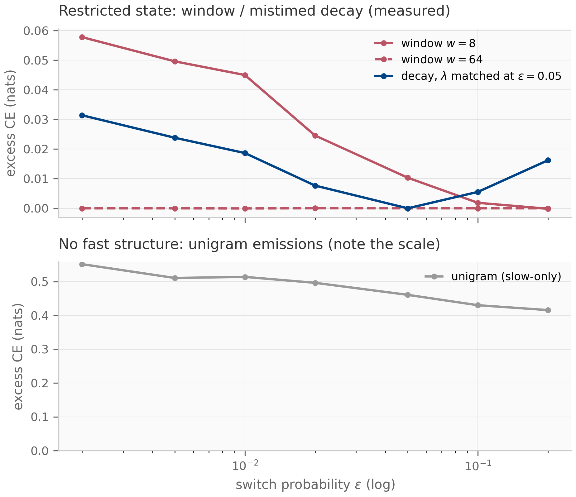
The third timescale, and the benchmark design lesson. The window curves above collapse to zero by $w = 64$. Why so small? Because with $\eta = 0.4$ the regimes are still locally distinguishable enough that a few dozen tokens identify the current regime — the identification timescale $\tau_{\mathrm{id}}$ is short. The overlap dial exists to control exactly this, and the crossover figure sweeps it:

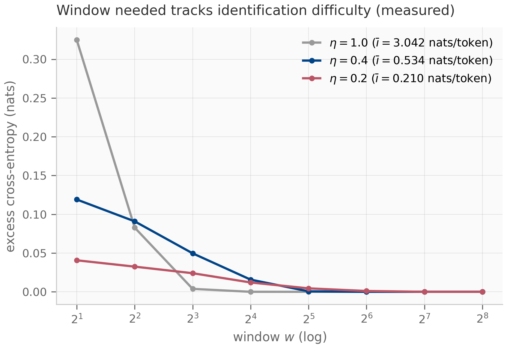
The design lesson is the section’s payload, and it is a constraint on benchmarks rather than on architectures: a two-timescale task separates fast-path from slow-path machinery only when the three timescales are ordered $w \ll \tau_{\mathrm{id}} \ll 1/\varepsilon$. Make the regimes too distinguishable ($\eta \to 1$) and a sliding window solves everything — the benchmark measures nothing about carried state. Make them too similar and even the optimal filter gains little — there is nothing to measure at all. Pilot B’s benchmark must therefore report $\bar{\imath}$ (or place $\tau_{\mathrm{id}}$ directly) as a task parameter alongside $\varepsilon$, exactly as this companion does. One measurement is deliberately deferred with the protocol: the composite restriction — a window-$w$ filter seeded at its edge with a decayed carried prior instead of the uniform one — is the idealized matched expansion itself, the natural probe of §14.2’s third leg, and it belongs with B’s protocol work rather than this chapter’s seed. What else does not transfer to Chapter 16 from here: the per-layer probing protocol that asks where a trained hybrid stores the regime posterior, the evaluation tiers around real benchmarks, and B’s five-axis decomposition — that is Chapter 16’s subject.

14.7 What’s next

This chapter mixed the layer families of Chapters 9–12 into hybrids and read the mixture through a fast–slow lens with one continuous theorem (Theorem 14.1) and one discrete one (Theorem 14.4) holding the interpretation to account. Its sibling beyond-SSM chapter, Chapter 13 (already behind you if reading in order), lives inside the gates themselves: exponential gating with its stabilizer states (xLSTM) and the generalized delta rule (RWKV-7) extend Chapter 12’s lineage to matrix memories with their own stability questions. Chapter 15 plays prosecution — the counter-evidence file on what SSM-heavy designs provably cannot do, and the diagnostic toolkit for detecting it. Chapter 16 builds the evaluation methodology this chapter’s benchmark seed feeds into — the protocol around the task, the per-layer probes, and the point where pilot B’s book-side prerequisites close.

14.8 Exercises

Three short problems (solutions inline) and three longer ones (solutions in §14.9).

Exercise 14.1 (short)

A 32-block hybrid has width $d = 2048$, window $w = 2048$, and ratio $7\!:\!1$ (so $n_a = 4$). Using Proposition 14.2, compute the decode state in floats, the same stack’s full-attention cache at $\seqlen = 131{,}072$, and the ratio. At what context length $\seqlen^\star$ does full attention’s cache equal the hybrid’s?

Exercise 14.2 (short, code)

Run companions/ch14/jax/two_timescale.py. Report the reference-configuration excesses (window-8, mistimed decay, unigram), then change _FIG_OVERLAP to $1.0$ and to $0.2$ and report how the window-8 excess at $\varepsilon = 0.005$ moves. One sentence: why does the hardest-to-identify task show the smallest window-8 excess?

Exercise 14.3 (short)

Let $a = \mathrm{attn}(x)$ and $s = \mathrm{ssm}(x)$ be the two branch outputs at one position, and suppose $a \ne s$ in every channel. Show that the set of outputs reachable by a scalar gate is a line segment in $\mathbb{R}^d$, that the vector-gate reachable set is the full axis-aligned box with corners $a$ and $s$, and conclude the dimension counts ($1$ versus $d$) behind Proposition 14.3.

Exercise 14.4 (theory) — solution in §14.9

Prove Theorem 14.1 in the scalar case $\dot{x} = ax + by$, $\varepsilon\dot{y} = cx + dy$ with $d < 0$: solve the $\eta = y + (c/d)x$ dynamics exactly, exhibit the boundary layer, and bound $|x - x_r|$ on $[0, T]$ explicitly, identifying where each hypothesis ($d < 0$, fixed $T$, bounded initial data) is used.

Exercise 14.5 (theory) — solution in §14.9

Prove Theorem 14.4, then compute the spectrum of $T(\varepsilon)$ and of $M(\lambda)$, the stationary distribution of each, and the mixing time of the regime chain. Conclude that for large $K$ the matched rate $\lambda^\star \approx \varepsilon$: forgetting toward uniform at the switching rate.

Exercise 14.6 (theory) — solution in §14.9

Complete the second strictness in Proposition 14.3: construct two inputs $x^{(1)}, x^{(2)}$ and a target map realizable by an input-dependent vector gate but by no constant vector gate. Then explain why a gate computed from another layer’s state (the GMU pattern) sits in the input-dependent class.

14.9 Full solutions to theory exercises

Solution to Exercise 14.4

With $\eta = y + (c/d)x$ the fast equation becomes, exactly as in the matrix case,

a scalar linear ODE with constant contraction rate $|d|/\varepsilon$ (here $d < 0$ is used — without it $\eta$ grows and there is no layer). Variation of constants:

On $[0, T]$ the trajectory $(x, y)$ is bounded uniformly in $\varepsilon$, say by $R$ — and this is where $d < 0$ earns its keep a second time. Fixed horizon and bounded data alone give only an $\varepsilon$-dependent bound (the system matrix has $O(1/\varepsilon)$ entries); with $d < 0$, the contraction keeps $|\eta(t)| \le |\eta(0)| + O(\varepsilon R)$, hence $|y| \le |c/d|\,|x| + |\eta(0)| + O(\varepsilon R)$, the slow equation then bounds $|x|$ by an $\varepsilon$-independent Grönwall constant, and a standard bootstrap (pick $R$ dominating both estimates; continuity keeps the trajectory inside) closes the loop. Without $d < 0$ the fast variable blows up as $\varepsilon \to 0$ and no uniform $R$ exists. With $R$ in hand, $|(ax + by)(s)| \le (|a| + |b|)R$, so the integral term is at most $\tfrac{|c|}{|d|}(|a| + |b|) R \cdot \tfrac{\varepsilon}{|d|}(1 - e^{dt/\varepsilon}) \le \tfrac{|c|(|a| + |b|) R}{d^2}\,\varepsilon$: the boundary-layer estimate $|\eta(t)| \le e^{-|d| t/\varepsilon}|\eta(0)| + O(\varepsilon)$, with the layer over by $t \sim \varepsilon\log(1/\varepsilon)$. Substituting $y = -(c/d)x + \eta$ into the slow equation gives $\dot{x} = (a - bc/d)x + b\eta$, so $e = x - x_r$ obeys $\dot{e} = (a - bc/d)e + b\eta$, $e(0) = 0$, and

where the fixed horizon $T$ is used to keep the Grönwall factor a constant. Each piece of the theorem’s statement appears with explicit constants. $\blacksquare$

Solution to Exercise 14.5

The identity. Diagonal entries: $T(\varepsilon)_{ii} = 1 - \varepsilon$ and $M(\lambda)_{ii} = 1 - \lambda + \lambda/K$; equality forces $\lambda(1 - 1/K) = \varepsilon$, i.e. $\lambda^\star = \varepsilon K/(K-1)$. Off-diagonal: $T_{ij} = \varepsilon/(K-1)$ and $M_{ij} = \lambda/K$, and at $\lambda^\star$ indeed $\lambda^\star/K = \varepsilon/(K-1)$. Both matrices are row-stochastic, so matching all entries matches the matrices; the constraint $\lambda^\star \le 1$ is $\varepsilon \le (K-1)/K$. Since the Bayes filter’s only use of the regime chain is the prior update $p \mapsto p\,T(\varepsilon)$, replacing $T$ by $M(\lambda^\star)$ changes nothing at any step: the fixed-decay filter at the matched rate is the Bayes filter, identically. $\blacksquare$

Spectra and mixing. Both matrices are of the form $\alpha I + \beta J$: eigenvalues $\alpha + K\beta$ on the all-ones vector and $\alpha$ on its $(K-1)$-dimensional complement. For $T(\varepsilon)$: eigenvalue $1$ (stochasticity) and $1 - \varepsilon - \varepsilon/(K-1) = 1 - \lambda^\star$ with multiplicity $K - 1$; for $M(\lambda)$: $1$ and $1 - \lambda$. The stationary distribution of each is uniform (both are doubly stochastic). The regime chain forgets its initial condition at geometric rate $1 - \lambda^\star$ per step — mixing time $\sim 1/\lambda^\star$ — which is the precise sense in which $1/\varepsilon$ is the slow timescale. As $K \to \infty$, $\lambda^\star = \varepsilon K/(K-1) \to \varepsilon$: forget toward uniform at exactly the switching rate. $\blacksquare$

Solution to Exercise 14.6

Take $d = 1$ (one channel suffices) and any two inputs with $a^{(1)} := \mathrm{attn}(x^{(1)}) \ne \mathrm{ssm}(x^{(1)}) =: s^{(1)}$ and likewise $a^{(2)} \ne s^{(2)}$. Define the target map to output the attention branch on $x^{(1)}$ and the SSM branch on $x^{(2)}$. A constant gate $g \in [0,1]$ must satisfy $g a^{(1)} + (1-g) s^{(1)} = a^{(1)}$, forcing $g = 1$, and $g a^{(2)} + (1-g) s^{(2)} = s^{(2)}$, forcing $g = 0$ — contradiction. An input-dependent gate with $g(x^{(1)}) = 1$, $g(x^{(2)}) = 0$ realizes the target, so the inclusion is strict. (With $d \ge 2$ the same argument runs per channel.)

A GMU-style gate is computed from the hidden state of another layer — a deterministic function of the network input — so as an input–output map it is exactly an input-dependent vector gate: $g = g(x)$, with the cross-layer sharing changing where the gate’s information comes from (a memory stream computed once and reused) but not the function class. That is why SambaY’s throughput gain is a systems gain — fewer recomputations of expensive context — while its expressivity class is the one already characterized here. $\blacksquare$

14.10 Companion code

The companions live in companions/ch14/{jax,torch} and are float64 throughout. The JAX modules are canonical and produce all four figures; the torch modules mirror the hybrid block and the filter family with cross-framework parity pinned to $< 10^{-9}$ (tokens drawn once and fed to both implementations). No Julia module this chapter: the numerical core is filtering linear algebra, not the integrator analysis that earned Julia its seat in Chapters 10 and 12.

# JAX (canonical; emits the four figures to public/figures/ch14/)
PYTHONPATH=. python companions/ch14/jax/hybrid_block.py
PYTHONPATH=. python companions/ch14/jax/two_timescale.py

# Tests: JAX identities (< 1e-12), torch parity (< 1e-9)
.venv/bin/pytest companions/ch14 -q

• hybrid_block.py — sliding-window attention with its per-position oracle, the gated-decay EMA and its closed form, the three composition patterns with exact gate reductions, the $r\!:\!1$ schedule, and the decode-cost accounting audited against materialized buffers; produces the cost-frontier and design-space figures (§§14.3–14.5).
• two_timescale.py — the two-timescale HMM with the overlap dial, the exact forward filter validated against brute-force path enumeration, the window / fixed-decay / unigram restrictions, the matched-decay identity at machine precision, and the discrimination diagnostic $\bar{\imath}$; produces the two-timescale-error and window-crossover figures (§§14.2, 14.6). This module is pilot B’s seed artifact.
• torch/ — eager mirrors of both modules plus the buffers-vs-Parameters distinction in a minimal gated-mix layer (the learned blend is a Parameter; the fixed decay rates are a buffer).