Exponential gates and matrix memory: xLSTM and RWKV-7
One generalized linear recurrence whose transition is diagonal-plus-rank-one — RWKV-7's generalized delta rule (rank-one removal in a learned direction, not the key) and xLSTM's matrix memory with exponential gating (and the log-domain stabilizer state that overflow forces) — extending Chapter 12's delta-rule lineage to matrix memories with their own stability questions.
On this page
- 13.1 The move: the gate inside the nonlinearity
- 13.2 The generalized transition and its spectrum
- 13.3 RWKV-7’s generalized delta rule
- 13.4 xLSTM: matrix memory and exponential gating
- 13.5 Stability, the trigger taxonomy, and the production lineup
- 13.6 What’s next
- 13.7 Exercises
- Exercise 13.1 (short)
- Exercise 13.2 (short, code)
- Exercise 13.3 (short, code)
- Exercise 13.4 (theory) — solution in §13.8
- Exercise 13.5 (theory) — solution in §13.8
- Exercise 13.6 (theory) — solution in §13.8
- 13.8 Full solutions to theory exercises
- Solution to Exercise 13.4
- Solution to Exercise 13.5
- Solution to Exercise 13.6
- 13.9 Companion code
Exponential gates and matrix memory: xLSTM and RWKV-7
13.1 The move: the gate inside the nonlinearity
Chapter 12 read a sequence layer’s state update as one step of an optimizer and organized the delta-rule family around a single linear recurrence,
with the state retrieved by and the transition acting on the right. Every architecture in that chapter shared one transition shape: — a scalar decay times the identity, minus a rank-one term locked to the write key . Gated DeltaNet’s was the only freedom beyond the delta rule, and it was a single number per step (Proposition 14.3 measures what that granularity costs).
Two threads were left open. Chapter 12 ended at the capacity wall (Proposition 11.4): a rank- state holds at most independent associations, and the delta rule erases interference without raising that ceiling. And its transition forgot only in the write direction — the orthogonal complement was inert, persistent memory that gradient flow on the current pair never cleans up. This chapter’s two architectures attack both by generalizing the transition itself, in two independent generalizations of the same linear recurrence:
- RWKV-7 Peng et al. (2025) keeps the rank-one shape but frees the removal direction and the diagonal: the erase direction need not be the key, and the decay is per-channel, not scalar. This is its “generalized delta rule,” and Chapter 12’s whole lineage falls out as a special case.
- xLSTM Beck et al. (2024) keeps a matrix memory and writes it with exponential gates — the input gate is , unbounded — which requires a stabilizer state to keep the recurrence inside float range.
The unifying object is the generalized transition
a diagonal decay (replacing Chapter 12’s scalar ) minus a rank-one removal in a unit direction (replacing the key-locked ). The rest of the chapter is two questions about this one matrix — when does it contract (§13.2), and what does freeing buy (§13.3) — followed by xLSTM’s exponential-gate variant and the stabilizer it forces (§13.4).
13.2 The generalized transition and its spectrum
Whether the recurrence keeps a bounded state is, as in Chapter 12, a question about the eigenvalues of the transition. The generalized is built from a diagonal and a symmetric rank-one term, so it is itself symmetric — and therefore has a real spectrum we can read exactly.
Let with a unit vector and . Then is symmetric, and:
- (Secular equation, interlacing.) Its eigenvalues are the for which , together with the roots of The rank-one downdate pushes every eigenvalue down without crossing the next diagonal entry, so the spectrum interlaces the sorted and lies in .
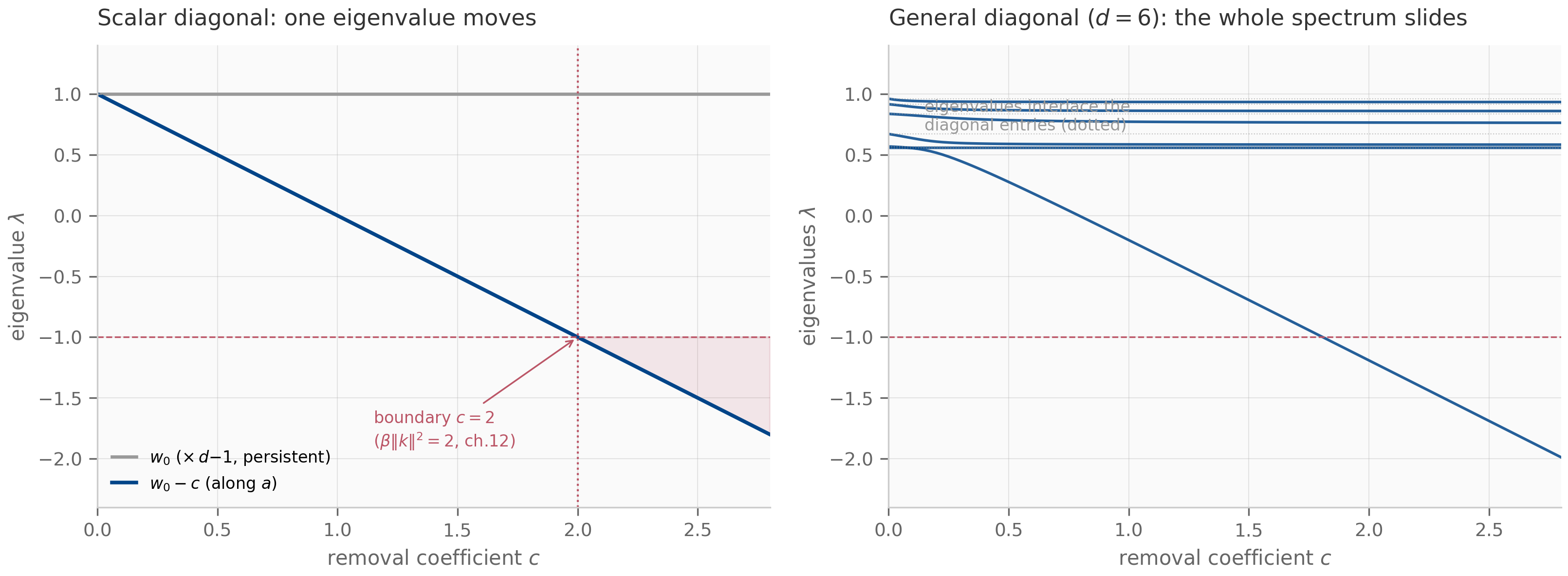
- (Scalar-diagonal case.) If , exactly one eigenvalue moves: the spectrum is , with spectral radius . At this is , recovering DeltaNet’s -direction radius (Theorem 12.4) under the identification — and the contractivity boundary is exactly forward Euler’s.
The proof is the matrix-determinant lemma: , so the roots of are the eigenvalues away from the
diagonal entries; the scalar case is the direct eigendecomposition of , whose only non- eigenvalue lies along (Exercise 13.4
carries the derivation). The companion reads the spectrum two ways — eigvalsh
of the materialized against the scalar-diagonal closed form — and they agree
to a measured ; the secular residual at the general-diagonal
eigenvalues is .
One reading of Proposition 13.1 matters for everything that follows. With a scalar diagonal at , the radius is : the transition is never strictly contractive, because the directions orthogonal to sit at eigenvalue exactly — Chapter 12’s inert persistent memory, unchanged. Strict contraction of those directions is what the diagonal buys: entries forget per-channel, the generalization of Gated DeltaNet’s single to a vector. Freeing the diagonal and freeing the removal direction are the two independent degrees of freedom RWKV-7 adds, and the spectrum shows they do different jobs — decay versus erasure.
13.3 RWKV-7’s generalized delta rule
RWKV-7 Peng et al. (2025) runs the generalized transition over a stream,
with a per-channel decay , a unit removal direction , a removal coefficient , and a write whose key is decoupled from . The paper’s own framing is “a newly generalized formulation of the delta rule with vector-valued gating and in-context learning rates” — and the precise sense in which it generalizes the delta rule is a one-line reduction.
Set (scalar diagonal), (removal direction = unit key), , and write . Then the generalized recurrence equals Gated DeltaNet’s update
identically. Hence plain DeltaNet () and the entire Chapter 12 lineage are the scalar-diagonal, removal-locked-to-the-key special case; RWKV-7’s added freedom is precisely the per-channel diagonal and the learned direction .
The proof substitutes and matches: , and the scalar
diagonal contributes the , so (Exercise 13.5). The companion runs the
generalized recurrence with these parameters against Chapter 12’s
gated_delta_recurrent and pins the difference at ; the
rank-one lax.scan form matches the materialized-transition Python-loop oracle
at .
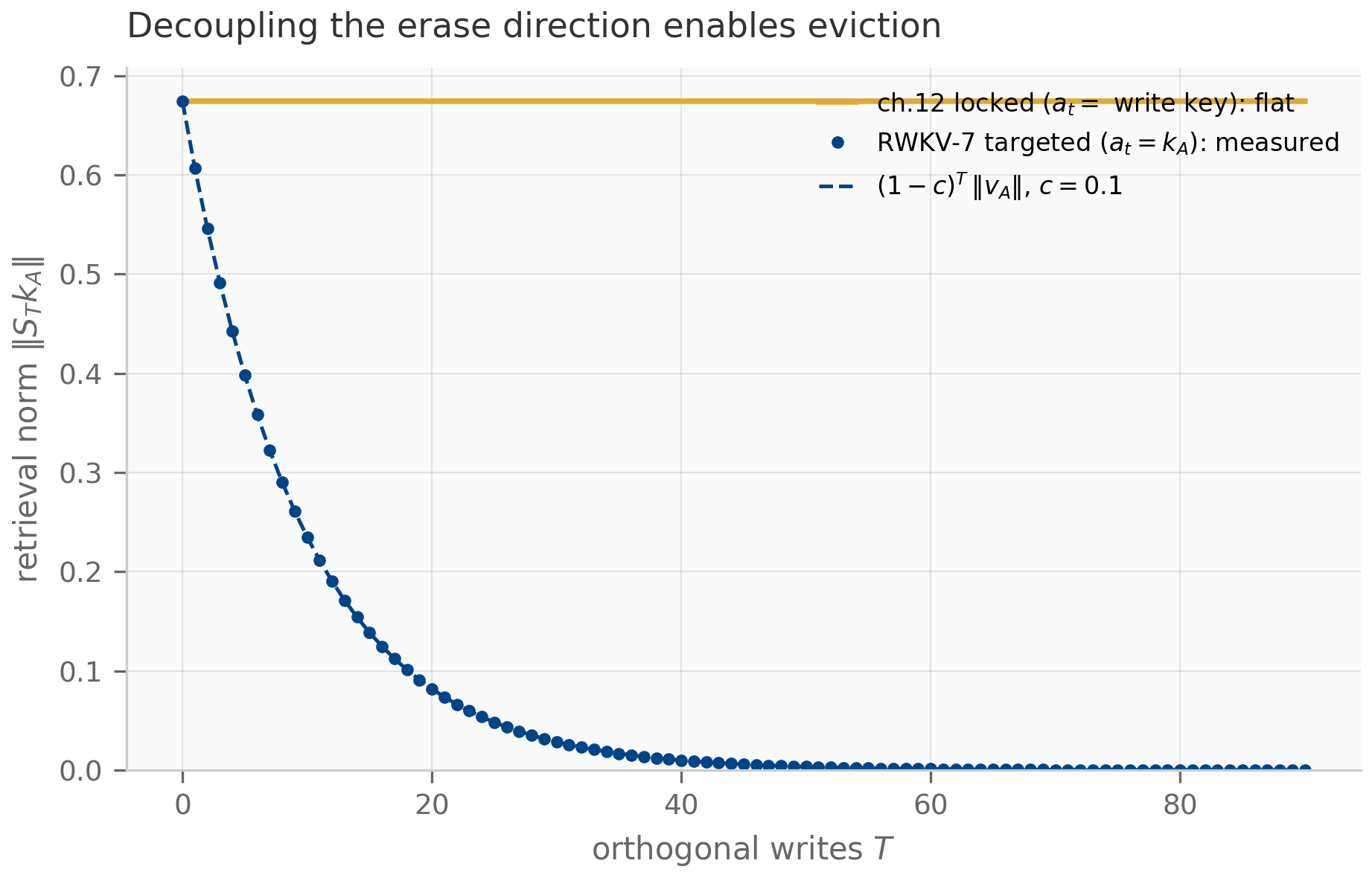
What does the learned direction buy, concretely? In Chapter 12 the only way to remove the association stored on a key was to write again with key — erasure was welded to the write. RWKV-7 can aim its rank-one removal at while writing some other, orthogonal pair, evicting the old association without overwriting it. Store on a unit key, then perform writes whose keys are orthogonal to :
- with the removal aimed at (direction , coefficient ), the retrieval decays as exactly — eviction with no overwrite;
- with the removal locked to the write key (Chapter 12’s ), the orthogonal writes never touch and — flat, the same inert-complement fact from §13.2.
The companion measures the decay at , as , matching to , against a flat locked baseline of . Decoupling the erase direction from the key is the whole content of “generalized” — and it is what lets RWKV-7 track state, not merely store associations.
13.4 xLSTM: matrix memory and exponential gating
xLSTM Beck et al. (2024) arrives at the same matrix recurrence from the LSTM side rather than the delta-rule side. Its mLSTM cell carries a matrix memory and a normalizer vector ,
written with scalar gates the architecture moves inside an exponential: the
forget gate is bounded, but the input gate
is not. An unbounded input gate is the deliberate
move: it lets a single high-surprise token’s write dominate the entire running
memory — a sharper, winner-take-more selectivity than any sigmoid can express.
(xLSTM’s other cell, sLSTM, applies the same exponential gates to a scalar memory
with a memory-mixing recurrence; the matrix mLSTM is this chapter’s subject.) That
expressivity is exactly the source of the problem: overflows
float64 once , and the naive recurrence then produces
inf/nan.
The fix is a stabilizer state, a running maximum carried in the log domain:
with which the gates are rescaled and the memory is carried in scaled coordinates , . This is the online-softmax running-max trick, and it is exact:
Let be the naive mLSTM states with raw gates , , and define the stabilized states , via the max-state above. Then:
- (Range.) The rescaled gates and lie in (because and by definition of the max), so the scaled recurrence never overflows.
- (Exactness.) The readout is invariant under the rescaling: The only change is that the floor becomes . Wherever the naive recurrence is finite the two agree to machine precision; where it overflows, the stabilized one stays finite and still correct.
Part 1 is the definition of the max; part 2 factors out of numerator
and denominator (Exercise 13.6). The one place the rescaling is visible is the
readout floor — the constant becomes — and getting that scaling
right is exactly what makes the stabilizer a change of variables rather than a
numerical approximation: it buys range and costs nothing in the answer. The
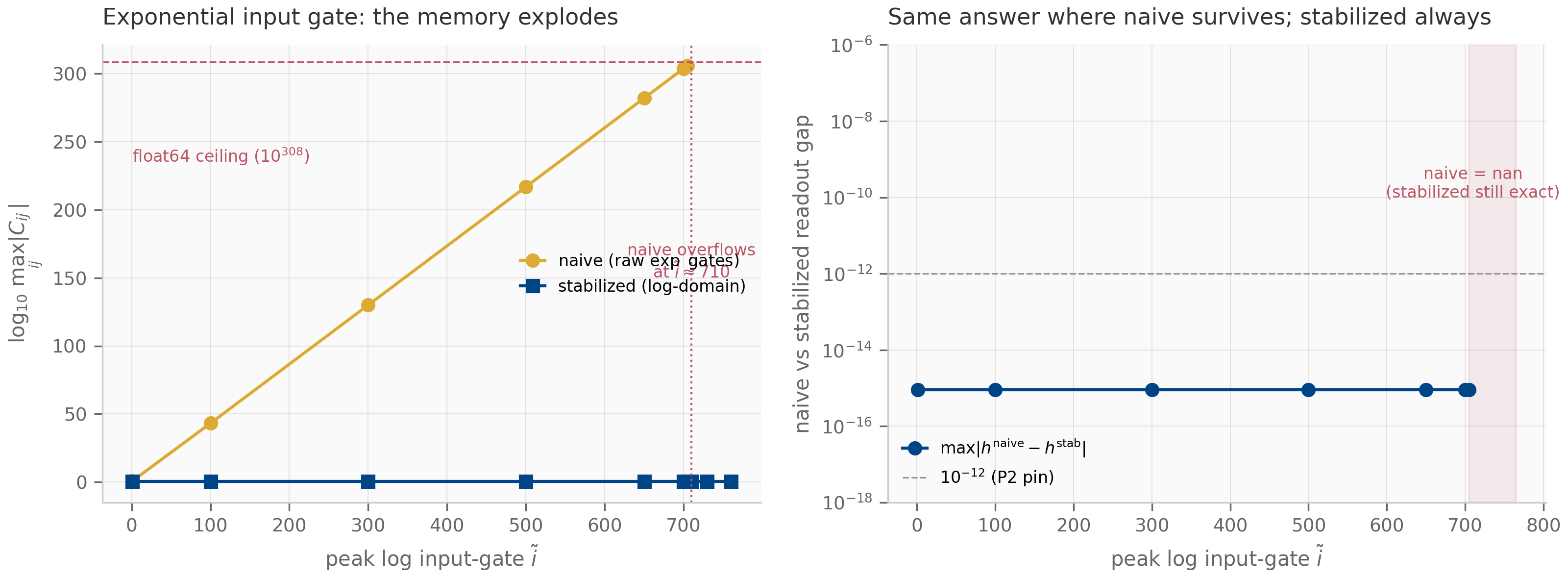
companion confirms both halves: in the safe regime the stabilized and naive
readouts agree to ; pushed to an input log-gate of ,
the naive memory reaches a peak entry of — finite, but a
hair from the ceiling — and the readouts still agree to ; at
the naive recurrence overflows ( of its readout entries become
nan), while the stabilized one stays bounded (peak entry ) and exact.
The cleanest statement of what the stabilizer guarantees is a recovery property. Store one pair on a unit key with input log-gate , then read at : the stabilized readout is exactly , for any . With one write, and with , so — the normalizer cancels the gate, which is what the exponential input gate is for. The companion stores the fixed pair and recovers it to even at , where the naive recurrence has long since overflowed; the Julia companion recovers the identical value, a cross-language anchor on the stabilized readout.
This is the book’s stability thread reappearing inside the architecture. Chapter 2 asked when a state stays bounded; Chapters 5–6 answered it for integrators with the explicit/implicit dichotomy, and Chapter 6’s implicit methods bought unconditional stability by solving rather than extrapolating (Proposition 6.1). xLSTM’s stabilizer is the same bargain made numerically: it does not change which mathematical object the recurrence computes, it changes the coordinates so the computation stays in range — an unconditional guarantee that the matrix memory never overflows, paid for with one extra scalar of state.
13.5 Stability, the trigger taxonomy, and the production lineup
Both architectures put a stability question inside the state — but in two different registers, and the difference is the point. RWKV-7’s is dynamical: the generalized transition contracts only when the diagonal decays and the rank-one removal stays within the boundary Proposition 13.1 draws — the explicit-method story from Chapter 12, now per-channel, a statement about the trajectory of the state. xLSTM’s is numerical: the exponential gate would overflow, and the max-state stabilizer is an in-state guarantee that it does not — not a claim about the dynamics at all, but about keeping the computation in float range, the implicit method’s unconditional-stability bargain made about representation rather than about the step. Chapter 15 returns to both with diagnostic tools (Lyapunov exponents, regime detection) that measure these stabilities on trained networks rather than asserting them at the architecture level.
There is a taxonomy worth closing here. Chapter 14 organized gates by what triggers a memory write — the input (content), the output, or a fixed layer schedule (Proposition 14.3). xLSTM’s exponential input gate is the sharpest input-triggered write in production. The remaining class is triggered by neither input nor position but by the model’s own loss: the Titans line Behrouz et al. (2025) writes to a neural long-term memory at test time, taking a gradient step on a surprise objective as it reads — a memory whose update rule is itself learned and fired by prediction error. That makes it a fourth trigger class (the loss), and it lives on a matrix memory of exactly the kind this chapter studies; its test-time-training mechanics are a distinct enough subject that this book names and places the trigger class here but does not pursue the test-time-training machinery further.
In production as of mid-2026 these are not toys: xLSTM has been trained at the B-parameter scale and RWKV-7 (“Goose”) at B, the latter reaching state-of-the-art multilingual performance at its size on dramatically fewer training tokens than comparable models Peng et al. (2025) . The diagonal-plus-rank-one transition and the exponential-gate stabilizer are not pedagogical simplifications — they are what these models run.
13.6 What’s next
Chapter 14 has already mixed these layers with attention into production hybrids, where the layer-ratio and gate-granularity decisions become design variables; Chapter 16 built the methodology that measures them honestly. The natural sequel to this chapter is Chapter 15, the counter-evidence file: it takes the stability questions raised here — when does a matrix memory’s recurrence stay bounded, and what can it provably not do — and turns them into diagnostics (Lyapunov exponents, effective state size) and impossibility results (the ceiling RWKV-7’s state-tracking claim brushes against). The generalized transition and the stabilizer state are the objects those diagnostics will probe.
13.7 Exercises
Exercise 13.1 (short)
For the scalar-diagonal transition (so , unit), use Proposition 13.1 to give the spectral radius at , , and . Which is non-contractive, and why is for every at this diagonal?
Solution
The spectrum is , so . At : . At : . At : — non-contractive (the iteration diverges, exactly forward Euler past its boundary). The radius is for every because the directions orthogonal to sit at eigenvalue : with the diagonal pinned at there is no per-channel decay, so the rank-one removal can shrink only the single direction . Strict contraction requires diagonal entries — the role of RWKV-7’s vector-valued .
Exercise 13.2 (short, code)
Run companions/ch13/jax/generalized_transition.py. Report the P3 reduction
error (generalized rule vs Chapter 12’s gated DeltaNet) and the decoupled-eviction
measurement at , : the targeted retrieval norm and the locked
baseline. What does the gap between them demonstrate?
Solution
The reduction error is — the generalized recurrence reproduces gated DeltaNet to machine precision, confirming Proposition 13.2. The eviction run reports targeted (matching to ) against a locked baseline of . The gap demonstrates the payoff of the learned direction: RWKV-7 can evict an old key by aiming its removal at it, while Chapter 12’s key-locked removal — under writes orthogonal to — leaves the association untouched. Decoupling the erase direction from the key is what “generalized” means.
Exercise 13.3 (short, code)
Run companions/ch13/jax/xlstm.py. Report the safe-regime readout gap between the
naive and stabilized recurrences, and the single-pair recovery error at input
log-gate . Why is the recovery error not affected by the gate’s magnitude?
Solution
The safe-regime readout gap is (the change-of-variables
exactness of Proposition 13.3), and single-pair recovery at
returns the stored value to — even though
overflows float64 and the naive recurrence is nan there. The
magnitude does not matter because the readout is a ratio: a single write makes
and with the same rescaled gate ,
and reading at gives . The
normalizer cancels the input gate exactly — which is precisely what an
unbounded input gate needs in order to be usable.
Exercise 13.4 (theory) — solution in §13.8
Prove part 1 of Proposition 13.1. Using the matrix- determinant lemma , derive the secular equation for the eigenvalues of away from the diagonal entries, and specialize to to recover the scalar-diagonal spectrum.
Exercise 13.5 (theory) — solution in §13.8
Prove Proposition 13.2. Substitute , , , into the generalized recurrence and show term-by-term that it equals Gated DeltaNet’s update. Identify which special case recovers plain DeltaNet, and which two degrees of freedom RWKV-7 adds over it.
Exercise 13.6 (theory) — solution in §13.8
Prove Proposition 13.3. (a) Show from the definition of . (b) By induction, show and where are the raw-gate states. (c) Conclude the readout identity, and explain why the constant floor must become rather than staying .
13.8 Full solutions to theory exercises
Solution to Exercise 13.4
Write and fix , so is invertible. Apply the matrix-determinant lemma with , , :
Since for , the eigenvalues there are exactly the roots of . (A diagonal entry is itself an eigenvalue iff , with eigenvector ; then the -term drops out of .) On each interval between consecutive distinct , is continuous and strictly monotone with poles of opposite sign at the endpoints, giving exactly one root per gap — the interlacing — and because shifts so that all roots lie at or below the corresponding , the spectrum sits in .
For : . Any vector orthogonal to is an eigenvector with eigenvalue (the rank-one term annihilates it), giving multiplicity ; and itself is an eigenvector, since . So the spectrum is and . At , , equal to once pushes the moving eigenvalue below ; with this is DeltaNet’s in the write direction, and exactly when .
Solution to Exercise 13.5
The generalized recurrence is . Substitute the four assignments. The diagonal term is . The rank-one term is
so . The write term is . Adding gives
which is exactly Gated DeltaNet’s update (Theorem 12.4). Setting (equivalently ) recovers plain DeltaNet, . The two degrees of freedom RWKV-7 adds over the lineage are (i) the per-channel diagonal in place of the scalar — vector-valued forgetting, the strict-contraction lever of §13.2 — and (ii) the learned removal direction , which decouples erasure from the write key (§13.3).
Solution to Exercise 13.6
(a) By definition , so and . Hence and , so and . Both are positive (exponentials) and at most .
(b) Induct on . At , and gives , consistent with the convention that the first write () discards the empty initial state. Assume . Then
using , . The identical computation gives .
(c) Substitute and into the naive readout:
The floor must scale to : the constant inside the naive lives in unscaled coordinates, and factoring out of the denominator divides it down to . Keeping the floor at in scaled coordinates would change the readout whenever the normalizer is small — the floor is the one place the change of variables is visible, and getting it right is what makes the stabilizer exact rather than approximate.
13.9 Companion code
The companions live in companions/ch13/{jax,torch,julia} and are float64
throughout; the JAX modules are canonical, the torch modules mirror their scoring
paths with cross-framework parity pinned , and the Julia module
cross-checks the stabilizer.
jax/generalized_transition.py— the diagonal-plus-rank-one transition, its spectrum (eigvalshagainst the scalar-diagonal closed form and the secular equation, Proposition 13.1), the generalized delta-rule recurrence (rank-onelax.scanvs a materialized-transition Python-loop oracle), the exact reduction to Chapter 12’s gated DeltaNet (Proposition 13.2), and the decoupled-eviction demo. Producestransition-spectrum.pngandlearned-direction.png.jax/xlstm.py— the mLSTM matrix-memory recurrence, the naive (overflow-prone) and log-domain-stabilized forms, the change-of-variables exactness (Proposition 13.3), the overflow cliff, and the single-pair recovery anchor. Producesstabilizer-overflow.png.torch/{generalized_transition,xlstm}.py— eager mirrors of the scoring paths, pinned to the JAX outputs intorch/tests/test_ch13_torch.py.julia/xlstm_stabilization.jl— a stdlib-only cross-language check of the stabilizer: the same P2 exactness, gate boundedness, overflow behavior, and the single-pair recovery of at input log-gate .
PYTHONPATH=. python companions/ch13/jax/generalized_transition.py
PYTHONPATH=. python companions/ch13/jax/xlstm.py
make companion-jax-tests          # all chapters' JAX suites
make companion-torch-tests        # JAX↔torch parity
julia --project=companions/ch13/julia companions/ch13/julia/runtests.jl