Discretization theory: ZOH, bilinear, exponential families

4.1 The discretization problem

Chapter 1 wrote the linear state-space system as a continuous-time ODE

defined for every $t \ge 0$. Computers do not handle “every $t$”; they handle a finite grid $t_k = k \stepsize$ for $k = 0, 1, 2, \ldots$ with step size $\stepsize > 0$. A discretization is a rule for building a recurrence

whose iterates $\statevec_k$ approximate the continuous trajectory at the grid points, $\statevec_k \approx \statevec(t_k)$. The two discrete matrices $\discA, \discB$ are functions of the continuous matrices $\statemat, \inputmat$ and of the step size $\stepsize$. Different functions give different discretizations.

There is no single canonical choice. Every discrete recurrence in this book — the S4 layer, the Mamba selective scan, the exp-trapezoidal scheme of Mamba-3 — picks a specific rule for translating $(\statemat, \inputmat, \stepsize) \mapsto (\discA, \discB)$. The choice matters: a poor discretization can take a perfectly stable continuous system and produce a discrete recurrence that diverges, fails to converge as $\stepsize \to 0$, or accumulates phase error on long horizons. Numerical-analysis textbooks Hairer et al. (1993) spend hundreds of pages on these failure modes. We will compress them into three properties and three schemes.

A useful warm-up is forward Euler, the simplest possible scheme:

This is what you get by replacing $\ddt \statevec$ with the forward difference $(\statevec_{k+1} - \statevec_k)/\stepsize$ and freezing the input at $u_k$. The discrete matrices are $\discA = I + \stepsize \statemat$ and $\discB = \stepsize \inputmat$. Forward Euler is the cleanest illustration of what can go wrong: it is only conditionally stable, meaning that for any fixed $\statemat$ with $\operatorname{Re}(\lambda_i) < 0$ there is a maximum step size beyond which $\discA = I + \stepsize \statemat$ acquires an eigenvalue of modulus $> 1$ and the recurrence blows up. The three schemes in §4.3–§4.5 fix this defect — each in its own way, with its own trade-off.

4.2 The Lax equivalence theorem

To compare schemes you need a definition of “correct.” The standard one comes from the Lax equivalence theorem Lax & Richtmyer (1956) , which decomposes correctness into two ingredients: consistency and stability.

A one-step scheme $\statevec_{k+1} = \Phi(\stepsize)(\statevec_k, u_k)$ is consistent with the ODE if its local truncation error — the residual you obtain by plugging the exact continuous trajectory into the discrete recurrence — vanishes faster than $\stepsize$ as $\stepsize \to 0$. Formally,

If $\tau(\stepsize) = O(\stepsize^p)$ the scheme is $p$-th order consistent. Higher $p$ means the per-step error shrinks faster with $\stepsize$.

A scheme is zero-stable if small perturbations $\delta$ injected at one step propagate boundedly to all future steps. For linear schemes this reduces to a uniform bound on the powers of $\discA$: there exists $K$ independent of $\stepsize$ such that $\norm{\discA^k} \le K$ for all $k$ with $k \stepsize \le T$, for any fixed horizon $T$. Equivalently, the spectral radius $\rho(\discA) \le 1 + O(\stepsize)$.

The two ingredients combine.

Convergence is what you actually want: that the discrete iterates approach the true continuous trajectory as you refine the grid. The theorem says you cannot get there by being consistent alone (you also need stability) or by being stable alone (you also need consistency). Both are necessary, and together they are sufficient. This is the convergence criterion every scheme in this chapter must pass.

For a stable LTI test problem — meaning $\statemat$ has all eigenvalues in the open left half-plane — there is a stronger notion sitting on top of zero-stability: a scheme is A-stable if $\rho(\discA) \le 1$ for every step size $\stepsize > 0$, not just for sufficiently small $\stepsize$. Forward Euler is not A-stable; ZOH, bilinear, and exp-trapezoidal are. The geometry of A-stability — the set of $\statemat \stepsize$ values for which the scheme behaves well — is the subject of Chapter 5.

4.3 Zero-order hold (ZOH)

The first scheme assumes the input is piecewise constant between samples: $u(t) = u_k$ for $t \in [t_k, t_{k+1})$. Under that assumption the inhomogeneous ODE solves exactly on a single interval. Starting from $\statevec(t_k) = \statevec_k$,

Identifying the two matrices,

This is the zero-order hold (ZOH) discretization. The hold refers to the input assumption; “zero-order” refers to the polynomial degree of the held signal (a constant is a zero-degree polynomial).

A practical wrinkle: writing $\discB$ as $\statemat^{-1}(e^{\statemat \stepsize} - I) \inputmat$ requires $\statemat$ to be invertible. The HiPPO matrix of Chapter 7 is invertible; some structured $\statemat$ in later chapters are not. The augmented matrix exponential trick handles both cases uniformly. Build the block matrix

where $P$ is the input dimension. Then

and a single expm call extracts both $\discA$ (top-left block) and $\discB$ (top-right block) without ever inverting $\statemat$. The S4 reference implementation uses this trick; so does the JAX companion discretization_comparison.py.

The proof is one line: $\abs{e^{\lambda_i \stepsize}} = e^{\operatorname{Re}(\lambda_i) \stepsize} < 1$ when $\operatorname{Re}(\lambda_i) < 0$ and $\stepsize > 0$. Stability is preserved for every positive step size, which is what A-stability means.

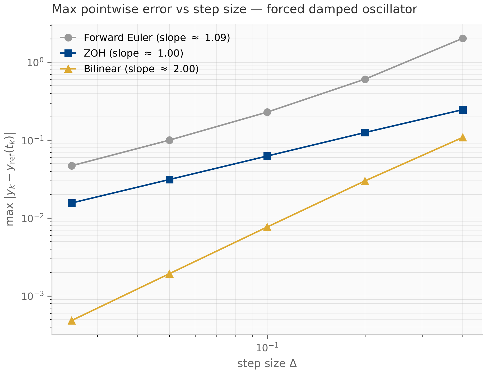
Two further properties are worth highlighting. First, for the autonomous ODE ($u \equiv 0$), ZOH is exact: the recurrence $\statevec_{k+1} = e^{\statemat \stepsize} \statevec_k$ matches $\statevec(t_{k+1}) = e^{\statemat \stepsize} \statevec(t_k)$ without any error at all. This is unusual — most discretizations have nonzero error even on autonomous systems. Second, for forced systems with smooth $u$, ZOH is first-order accurate: the per-step error in the forcing integral is $O(\stepsize^2)$ (because the integrand $e^{\statemat (t_{k+1} - s)} \inputmat (u(s) - u_k)$ is $O(\stepsize)$ over an interval of length $\stepsize$), and after $T/\stepsize$ steps the cumulative error is $O(\stepsize)$. The empirical convergence rate plotted in the companion log-log error figure confirms slope $\approx 1$.

4.4 The bilinear (Tustin) transform

The second scheme drops the piecewise-constant assumption and instead approximates the integral on $[t_k, t_{k+1}]$ by the trapezoidal rule: $\int_{t_k}^{t_{k+1}} f(s) \, ds \approx \tfrac{\stepsize}{2}(f(t_k) + f(t_{k+1}))$. Applied to the inhomogeneous ODE this gives an implicit recurrence,

which one solves for $\statevec_{k+1}$:

Reading off $\discA$ and $\discB$,

This is the bilinear transform, also called the Tustin transform after Arnold Tustin’s 1947 paper introducing it in control theory Tustin (1947) . The S4D paper uses bilinear discretization; so do many signal-processing toolboxes.

The bilinear formula has a striking geometric interpretation. Restricted to a single eigenvalue $\lambda$ of $\statemat$ (commuting through the simultaneous diagonalization), the map $\lambda \mapsto \mu$ that sends a continuous eigenvalue to its discrete image is

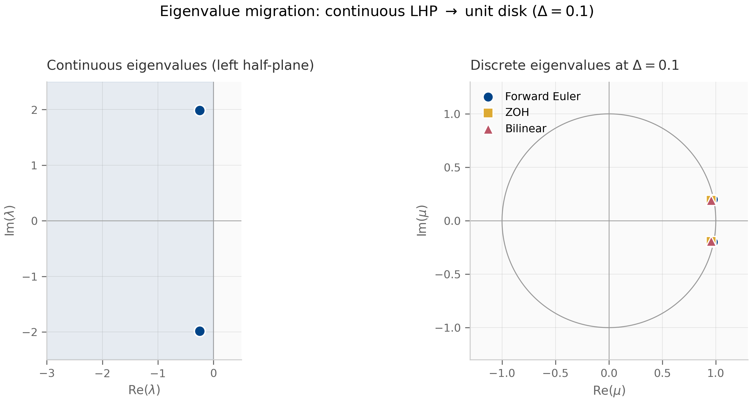
This is a Möbius transformation (a.k.a. fractional linear transformation) of the complex plane: $z \mapsto (az+b)/(cz+d)$ with $ad - bc \ne 0$. Möbius transformations are conformal — angle-preserving — and they map circles-or-lines to circles-or-lines. The specific Möbius map above sends the imaginary axis exactly to the unit circle and sends the open left half-plane exactly to the open unit disk.

The proof is geometric: $z := \tfrac{\stepsize}{2}\lambda_i$ has $\operatorname{Re}(z) < 0$, and $\abs{1+z} < \abs{1-z}$ iff $\operatorname{Re}(z) < 0$ (square both sides and cancel). Algebraically, $\abs{(1+z)/(1-z)}^2 = \abs{1+z}^2/\abs{1-z}^2 < 1$, which is exactly $\abs{\mu_i} < 1$. The full proof, with the Möbius geometry spelled out, is Exercise 4.5 in §4.9.

Bilinear is second-order accurate for smooth forcing — the trapezoidal-rule local truncation error is $O(\stepsize^3)$, giving global error $O(\stepsize^2)$. Unlike ZOH, it is not exact even on autonomous systems: the $(I - \tfrac{\stepsize}{2}\statemat)^{-1}(I + \tfrac{\stepsize}{2}\statemat)$ Padé approximation of $e^{\statemat \stepsize}$ agrees with the true exponential only through second order. The trade is one of structure: bilinear maps the imaginary axis exactly to the unit circle, so marginally stable continuous modes (purely imaginary eigenvalues) become marginally stable discrete modes (eigenvalues exactly on the unit circle). ZOH crushes them to the unit-disk interior at rate $e^{0 \cdot \stepsize} = 1$ (marginal in the limit but never exactly on the circle for finite $\stepsize$). This makes bilinear the natural choice when the system has oscillatory modes you want to preserve — a property that becomes load-bearing for the symplectic methods of Chapter 6.

4.5 Exponential-family discretizations

The third family takes a different approach: rather than approximating $e^{\statemat \stepsize}$ by a low-order Padé form (as bilinear does) or by the identity-plus-linear truncation $I + \stepsize \statemat$ (as forward Euler does), it computes $e^{\statemat \stepsize}$ exactly and approximates only the forcing integral. This is the philosophy of exponential integrators Hochbruck & Ostermann (2010) .

The exact one-step formula from variation of parameters (Chapter 1, §1.6) is

ZOH approximates $u(t_k + s) \approx u_k$ on $[0, \stepsize]$; bilinear approximates the integral by the trapezoidal rule with a Padé-approximated exponential. The exponential-trapezoidal scheme keeps the exact exponential and uses a linear interpolation of the input: $u(t_k + s) \approx u_k + (s/\stepsize)(u_{k+1} - u_k)$. Substituting and evaluating the resulting two integrals gives

where $\varphi_1$ and $\varphi_2$ are the first two $\varphi$-functions of the exponential family:

Both are entire functions (the apparent singularities at $z = 0$ are removable: $\varphi_1(0) = 1$, $\varphi_2(0) = 1/2$). Applied to the matrix $\statemat \stepsize$, they produce matrix-valued objects $\varphi_1(\statemat \stepsize), \varphi_2(\statemat \stepsize)$ that can be computed via the same augmented-matrix-exponential trick as ZOH.

Reading off the discrete matrices in the form $\statevec_{k+1} = \discA \statevec_k + \discB_0 u_k + \discB_1 (u_{k+1} - u_k)$:

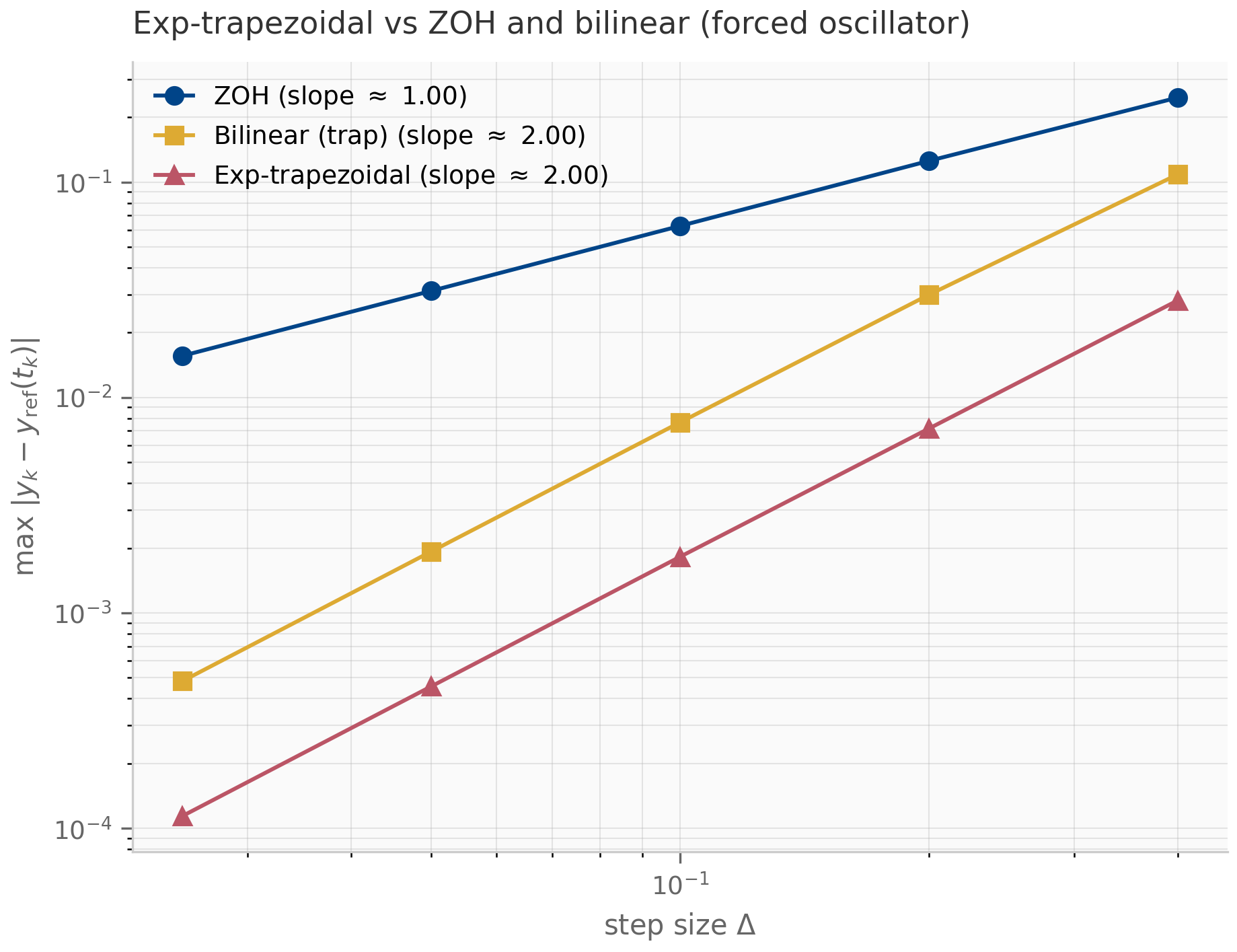
Notice that $\discA$ is the same as ZOH, so exp-trapezoidal preserves stability identically to ZOH: A-stable, exact for autonomous systems, eigenvalues in the unit disk for any $\stepsize > 0$. The improvement is in the order of accuracy: by interpolating $u$ linearly rather than holding it constant, exp-trapezoidal becomes second-order accurate (provided $u$ is $C^1$).

Exp-trapezoidal is the discretization of choice when the continuous dynamics are stiff — when $\statemat$ has eigenvalues with very different magnitudes, so the linear part is the hard part of the problem. By treating $e^{\statemat \stepsize}$ exactly the scheme sidesteps the step-size restriction that explicit methods inherit from the stiff eigenvalues, and the matrix exponential is computed once per layer in practice. Chapter 10 returns to this story for Mamba-3, which adopts exp-trapezoidal precisely because the input-dependent $\statemat(u_t)$ in selective SSMs produces stiff dynamics that ZOH and bilinear handle poorly.

A subtle implementation point: $\varphi_2(\statemat \stepsize)$ is not numerically equal to $(e^{\statemat \stepsize} - I - \statemat \stepsize)/(\statemat \stepsize)^2$ when this formula is computed naively, because catastrophic cancellation in the numerator destroys precision for small $\stepsize$. The standard remedy is to compute all $\varphi$-functions simultaneously from one augmented matrix exponential, again using the trick that produced $\discB$ for ZOH. Both companions (exp_trapezoidal.py in JAX and discretization_atlas.jl in Julia) implement the augmented form.

4.6 Order of accuracy and the discretization hierarchy

The three schemes are summarized in the table below. “Autonomous-exact” means the scheme produces zero error for the homogeneous problem ($u \equiv 0$). “A-stable” means $\rho(\discA) \le 1$ for every $\stepsize > 0$ on every stable LTI test problem.

The empirical order can be read directly off a log-log plot of error against step size: a $p$-th-order scheme has error $\propto \stepsize^p$, so on a log-log plot the data lie on a line of slope $p$. The Julia companion discretization_atlas.jl runs this sweep against a high-accuracy Tsit5 reference solution from DifferentialEquations.jl; the JAX companion discretization_comparison.py performs the same sweep using scipy.integrate.solve_ivp (Radau) as the reference.

The hierarchy is not strict: ZOH’s autonomous-exactness can outweigh its first-order accuracy when the forcing is mild relative to the homogeneous decay. Bilinear’s exact imaginary-axis preservation can outweigh its non-exactness on autonomous problems when the system has long-lived oscillations. Exp-trapezoidal combines the best of both — exact on autonomous, second-order on forced — at the cost of computing more $\varphi$-functions per step. The trade-offs are recurring themes throughout the SSM literature: S4 uses ZOH for its simplicity and exactness on the (autonomous) HiPPO drift; S4D and S5 follow suit; Mamba-3 switches to exp-trapezoidal once the input-dependence makes the dynamics stiff enough that the second-order error compounding matters.

4.7 What’s next

This chapter introduced three schemes and proved each preserves Lyapunov stability. Chapter 5 zooms in on the stability region of each scheme — the set of $\statemat \stepsize$ values for which $\rho(\discA) \le 1$ — and develops the Butcher-tableau machinery for systematically constructing higher-order Runge–Kutta methods. Chapter 6 then asks what to do when even A-stability is not enough — when the system is stiff or Hamiltonian and you need L-stable implicit methods, or symplectic methods that preserve geometric invariants. The exp-trapezoidal scheme of §4.5 turns out to be a member of a much larger family of exponential integrators, all of which deserve a place in your numerical-analysis toolkit.

Forward-looking SSM connections: ZOH is the default in Chapters 7–9 (HiPPO, S4, S4D, S5, Mamba-1/2). Bilinear shows up in S4D when the HiPPO matrix is diagonalized. Exp-trapezoidal is the Mamba-3 scheme, treated in Chapter 10.

4.8 Exercises

Six problems mixing computation and theory. Short/numerical (4.1–4.3) have inline collapsible solutions; long/proof exercises (4.4–4.6) have full worked solutions in §4.9.

Exercise 4.1 (computation)

Compute $\discA$ for ZOH on the 1-D test problem $\statemat = -2$, $\inputmat = 1$, $\stepsize = 0.1$. Then verify by hand that $\abs{\discA} < 1$.

Exercise 4.2 (computation)

Compute $\discA$ for the bilinear transform on the same 1-D problem ($\statemat = -2$, $\stepsize = 0.1$). Compare $\abs{\discA}_{\text{bilinear}}$ against $\abs{\discA}_{\text{ZOH}} = e^{-0.2}$ — which is smaller, and why?

Exercise 4.3 (computation + code)

Run companions/ch04/jax/discretization_comparison.py and verify empirically that ZOH has slope $\approx 1$ on the log-log error-vs-$\stepsize$ plot, bilinear and exp-trapezoidal have slope $\approx 2$. What happens to the ZOH slope if you set the forcing $u(t) \equiv 0$ (autonomous case)?

Exercise 4.4 (theory) — solution in §4.9

Prove the augmented matrix exponential trick used in §4.3: that

for invertible $M_1$, by computing the series term-by-term.

Exercise 4.5 (theory) — solution in §4.9

Prove that the Möbius transformation $z \mapsto (1 + z/2)/(1 - z/2)$ sends the open left half-plane $\set{z : \operatorname{Re}(z) < 0}$ bijectively to the open unit disk $\set{w : \abs{w} < 1}$, and sends the imaginary axis bijectively to the unit circle (minus the point $w = -1$).

Exercise 4.6 (theory) — solution in §4.9

Derive the exponential-trapezoidal scheme of §4.5 from the variation-of-parameters formula by substituting the linear interpolation $u(t_k + s) = u_k + (s/\stepsize)(u_{k+1} - u_k)$ into the forcing integral and evaluating term-by-term using the $\varphi$-function identities.

4.9 Full solutions to theory exercises

Solution to Exercise 4.4

The matrix $M := \begin{pmatrix} M_1 & M_2 \\ 0 & 0 \end{pmatrix}$ satisfies, for $k \ge 1$,

This is verified by induction: $M^1$ matches by construction, and $M^{k+1} = M \cdot M^k = \begin{pmatrix} M_1 & M_2 \\ 0 & 0 \end{pmatrix} \begin{pmatrix} M_1^k & M_1^{k-1} M_2 \\ 0 & 0 \end{pmatrix} = \begin{pmatrix} M_1^{k+1} & M_1^k M_2 \\ 0 & 0 \end{pmatrix}$ as required. Now sum the matrix-exponential series:

where $S := \sum_{k \ge 1} M_1^{k-1}/k! = M_1^{-1} \sum_{k \ge 1} M_1^k / k! = M_1^{-1}(e^{M_1} - I)$, using invertibility of $M_1$ to extract the leading $M_1^{-1}$. Plugging back gives the claimed result. ∎

This is exactly the identity used to compute $\discA$ and $\discB$ jointly from one expm call in §4.3: take $M_1 = \statemat \stepsize$ and $M_2 = \inputmat \stepsize$.

Solution to Exercise 4.5

Let $T(z) := (1 + z/2)/(1 - z/2)$. Imaginary axis to unit circle: for $z = i\omega$ with $\omega \in \R$,

so $T(i\omega)$ lies on the unit circle. The map $\omega \mapsto T(i\omega)$ traces the unit circle once as $\omega$ ranges over $\R$, missing only the limit point $T(\infty) = -1$.

Left half-plane to unit disk: write $z = x + iy$ with $x < 0$. Then

Since $x < 0$, $\abs{1 + x/2} < \abs{1 - x/2}$ (both for $\abs{x} < 2$ where the signs match the absolute values, and for $\abs{x} > 2$ where they reverse). The $y$-terms are identical in numerator and denominator. Therefore the numerator is strictly less than the denominator, so $\abs{T(z)} < 1$.

Bijectivity: Möbius transformations $z \mapsto (az + b)/(cz + d)$ with $ad - bc \ne 0$ are bijections of the Riemann sphere $\C \cup \set{\infty}$ to itself. Restriction to the half-plane gives a bijection to the disk. The inverse is $w \mapsto (2(w-1))/(w+1)$, which can be verified by direct computation. ∎

This Möbius geometry is the algebraic content of A-stability for bilinear: a scheme is A-stable iff its eigenvalue map sends the open left half-plane into the closed unit disk. Bilinear achieves this bijectively; ZOH does so as well but non-bijectively (it folds an infinite strip of width $2\pi/\stepsize$ onto the unit disk, aliasing high-frequency continuous modes onto low-frequency discrete ones).

Solution to Exercise 4.6

Start from variation of parameters on $[t_k, t_{k+1}]$:

Substitute the linear interpolant $u(t_k + s) = u_k + (s/\stepsize)(u_{k+1} - u_k)$ for $s \in [0, \stepsize]$:

with $I_0 := \int_0^{\stepsize} e^{\statemat (\stepsize - s)} \inputmat \, ds$ and $I_1 := \int_0^{\stepsize} \tfrac{s}{\stepsize} e^{\statemat (\stepsize - s)} \inputmat \, ds$. Change variables $\sigma = \stepsize - s$ in $I_0$:

where in the last step we substituted the definition $\varphi_1(z) = (e^z - 1)/z$ applied with argument $\statemat \stepsize$. For $I_1$, change variables again $\sigma = \stepsize - s$, so $s = \stepsize - \sigma$ and $s/\stepsize = 1 - \sigma/\stepsize$:

The remaining $\sigma$-weighted integral evaluates via integration by parts to $\statemat^{-2}(e^{\statemat \stepsize}(\statemat \stepsize - I) + I) \inputmat = \stepsize^2 \varphi_2(\statemat \stepsize) \inputmat$, using the $\varphi_2(z) = (e^z - 1 - z)/z^2$ identity. Carefully tracking the algebra gives $I_1 = \stepsize \, \varphi_2(\statemat \stepsize) \, \inputmat$ as claimed. Combining,

The local truncation error is $O(\stepsize^3)$ for $C^1$ inputs (the linear interpolation has error $O(\stepsize^2)$ over an interval of length $\stepsize$, and the integral picks up an additional $\stepsize$ factor). Global error is therefore $O(\stepsize^2)$ — second-order, as advertised.

4.10 Companion code

Three runnable companions for Chapter 4:

JAX (companions/ch04/jax/):

• discretization_comparison.py — implements ZOH, bilinear, and forward Euler in JAX; runs the error-vs-step-size sweep on a forced damped oscillator; emits eigenvalue_migration.png and order_convergence.png.
• exp_trapezoidal.py — implements the exp-trapezoidal scheme via the augmented matrix exponential; verifies second-order convergence against the same forced oscillator; emits exp_trap_convergence.png.

Julia (companions/ch04/julia/):

• discretization_atlas.jl — ports the post_transformers Week-9 reference implementation to ssm-foundations; uses DifferentialEquations.jl Tsit5 as the ground-truth reference solver and reports the empirical slope per scheme.
• Project.toml / Manifest.toml — companion-local Julia environment pinning DifferentialEquations and LinearAlgebra.

To run from the repo root:

# JAX (uses post_transformers .venv with scipy, numpy, matplotlib, jax pre-installed)
PYTHONPATH=. python companions/ch04/jax/discretization_comparison.py
PYTHONPATH=. python companions/ch04/jax/exp_trapezoidal.py

# Julia (first run will precompile DifferentialEquations.jl; ~2–5 minutes)
julia --project=companions/ch04/julia companions/ch04/julia/discretization_atlas.jl

All figures emit to public/figures/ch04/.