Mamba-3 and the exponential-trapezoidal integrator
How Mamba-3 keeps selectivity and changes two things — a second-order exponential-trapezoidal integrator and a complex state — turning the dynamical-systems lens of Chapters 4-6 onto a production sequence model.
On this page
- 10.1 Two upgrades to the selective SSM
- 10.2 The exponential-trapezoidal scheme
- 10.3 Stability and accuracy decouple
- 10.4 Complex state: decay and oscillation in one head
- 10.5 The trapezoidal SSD pass
- 10.6 MIMO and the production block
- 10.7 What’s next
- 10.8 Exercises
- Exercise 10.1 (short)
- Exercise 10.2 (short, code)
- Exercise 10.3 (short)
- Exercise 10.4 (theory) — solution in §10.9
- Exercise 10.5 (theory) — solution in §10.9
- Exercise 10.6 (theory) — solution in §10.9
- 10.9 Full solutions to theory exercises
- Solution to Exercise 10.4
- Solution to Exercise 10.5
- Solution to Exercise 10.6
- 10.10 Companion code
Mamba-3 and the exponential-trapezoidal integrator
10.1 Two upgrades to the selective SSM
Chapter 9 built the selective SSM: input-dependent make the dynamics linear time-varying, the convolution view collapses, and the selective scan plus the semiseparable-matrix view (SSD) carry the computation. Mamba-1 and Mamba-2 both discretize with zero-order hold (ZOH) and keep a real diagonal state matrix .
Mamba-3 Lahoti et al. (2026) changes two things of dynamical-systems substance and leaves the rest of the SSD scaffold (the semiseparable structure of Theorem 9.4, the scan, the attention duality of Theorem 9.5) intact:
- A second-order integrator. ZOH is first-order accurate; Mamba-3 adopts a second-order exponential-trapezoidal scheme — the exponential-integrator idea of Chapter 4 §4.5 in its trapezoidal-quadrature form (§10.2) — while keeping ZOH’s exact treatment of the homogeneous dynamics (§10.2-10.3).
- A complex state. A real diagonal mode can only decay; a complex mode decays and rotates, so a single head becomes a damped oscillator (§10.4).
Both changes are dynamical-systems moves, and both have been waiting since the foundations chapters: the integrator is the Chapter 4-5 story applied to a real architecture, and the complex state is the spiral phase portrait of Chapters 1-2. The C1 pilot’s empirical question — whether a second-order, structure-preserving integrator actually buys accuracy on a selective SSM without costing stability — is the through-line.
10.2 The exponential-trapezoidal scheme
Recall the continuous mode , whose exact one-step map is . Every exponential integrator keeps the transition exact (the philosophy of Chapter 4 §4.5) and approximates only the forcing integral. ZOH holds the input constant at the left endpoint; the exponential-trapezoidal scheme applies the trapezoidal quadrature rule to the forcing integral — averaging the integrand at the two endpoints. The integrand is at and at , so the rule gives . Weighting the two endpoints by gives the three-term update
The contrast with ZOH is the third term: where ZOH reads only the left endpoint , the trapezoid reads both endpoints. At this is the symmetric trapezoidal rule (globally second-order); at it collapses to a shifted ZOH (first order). Mamba-3 makes itself input-dependent (a sigmoid of a learned projection), one more selective knob.
This single fact — that is identical for the two schemes — has a sharp consequence for how the order can be measured.
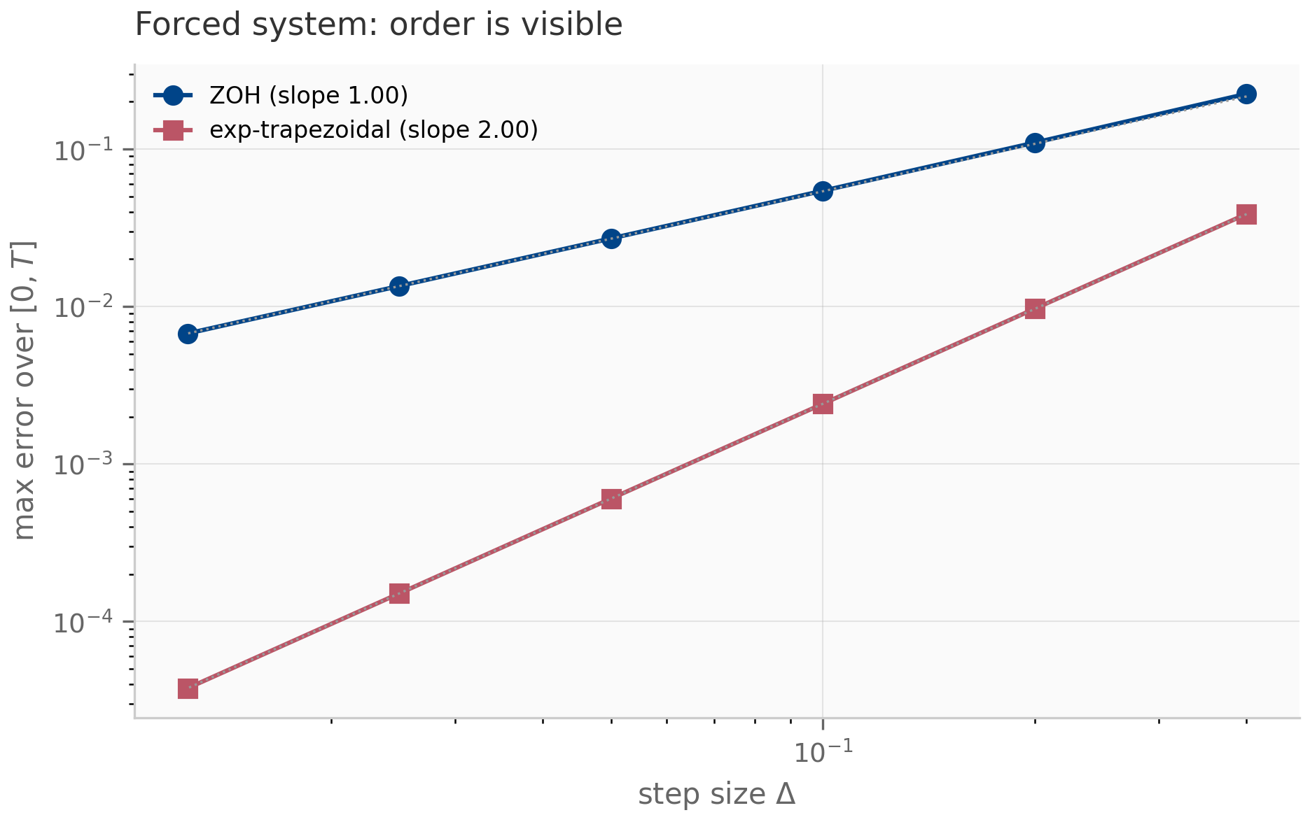
For the exponential-trapezoidal scheme has local truncation error per step, hence global order 2, provided the input is non-constant and . On the homogeneous system () both ZOH and exp-trapezoidal reproduce the exact solution to machine precision, so the order difference is unobservable there.
The proof is Exercise 10.4 (§10.9). The practical reading is a trap worth naming: because the homogeneous transition is exact, a convergence study run on an autonomous system shows ZOH and exp-trapezoidal as identical lines at roundoff — the second order is simply not visible. The companion confirms this directly: on the autonomous mode both schemes sit at , while on the forced mode the fitted convergence slopes separate cleanly into (ZOH) and (exp-trapezoidal). This is the same lesson Chapter 4 flagged in Exercise 4.3 (“setting makes ZOH exact; the slope is meaningless”), now load-bearing for verifying a real architecture’s headline claim.
10.3 Stability and accuracy decouple
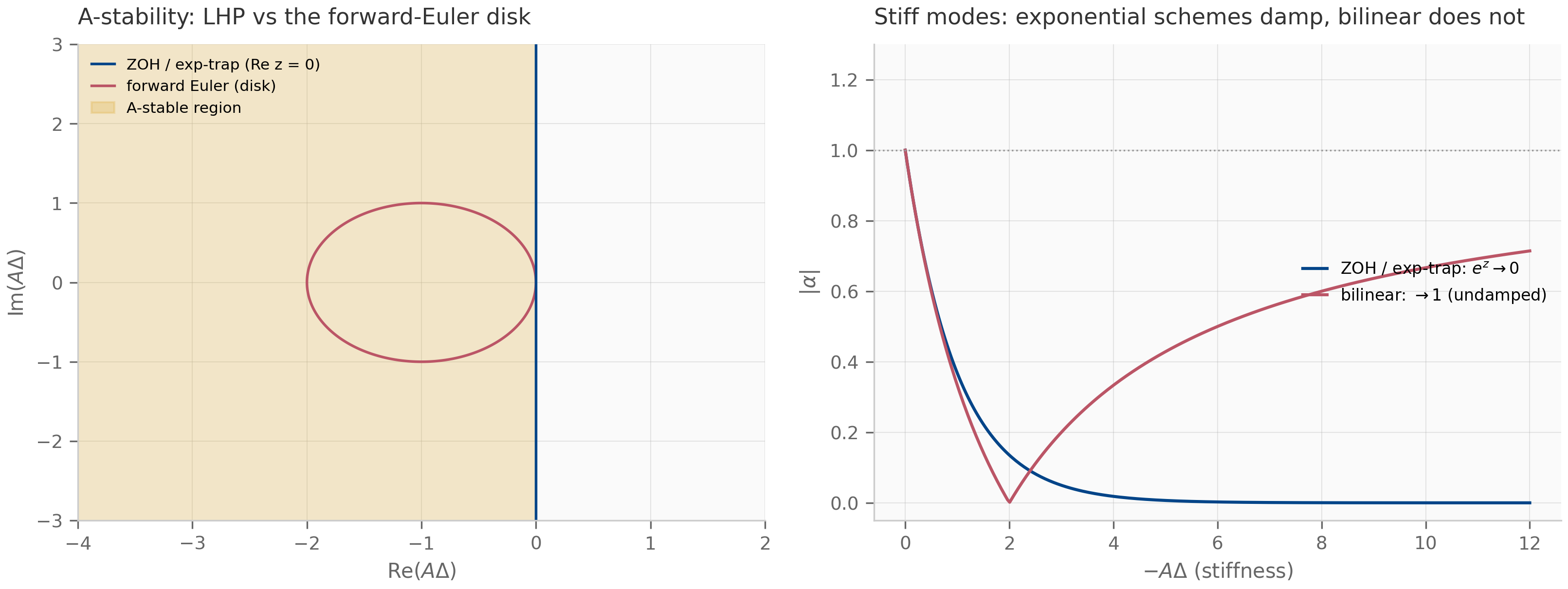
Why adopt an exponential integrator rather than a higher-order Runge-Kutta method? Because the exponential transition is exact, the discrete amplification factor is , which is for any stable mode () at any step size. ZOH and exp-trapezoidal are therefore unconditionally stable on the homogeneous part — A-stable over the entire left half-plane — and, crucially, stability is set by alone, independent of the order of the forcing quadrature. For a Runge-Kutta method a single stability polynomial controls both accuracy and the stability region; the exponential integrator decouples them.
For , the exponential-trapezoidal (and ZOH) amplification factor satisfies for every , and as the mode stiffens (). The bilinear (Tustin) scheme is also A-stable but uses the -Padé approximation , for which as the mode stiffens: stiff modes are left undamped.
The proof is Exercise 10.6 (§10.9). The companion makes the contrast quantitative: at a stiff , the exponential schemes give (fully damped) while bilinear gives (still ringing). This is why an exponential integrator is the right tool when the input-dependent of a selective SSM produces stiff dynamics, as Chapter 4 §4.5 anticipated for exactly this chapter. One caveat matters for §10.4: the theorem bounds the magnitude only. For a complex mode it says nothing about how faithfully the discrete rotation tracks the continuous phase — phase fidelity is a separate question, and the open one the frontier paragraph below raises.
The geometric-integrator frontier (where the pilot goes next). Exp-trapezoidal is a second-order exponential integrator; it is not symplectic. For the oscillatory complex modes introduced in §10.4, the question the symplectic-integrator pilot asks is whether a geometric integrator (Chapter 6) — one that preserves a phase-space invariant rather than merely a damping bound — controls long-horizon phase error better than exp-trapezoidal does. That is an open empirical question, not a settled result, and it is the heart of the “discretization stability atlas” the pilot pursues; Chapter 17 returns to it. This chapter establishes the settled part: exp-trapezoidal is second-order, A-stable, and exact on the homogeneous part.
10.4 Complex state: decay and oscillation in one head
A real diagonal mode gives : pure geometric decay, a single forgetting timescale. Mamba-3 lets the mode be complex, , so
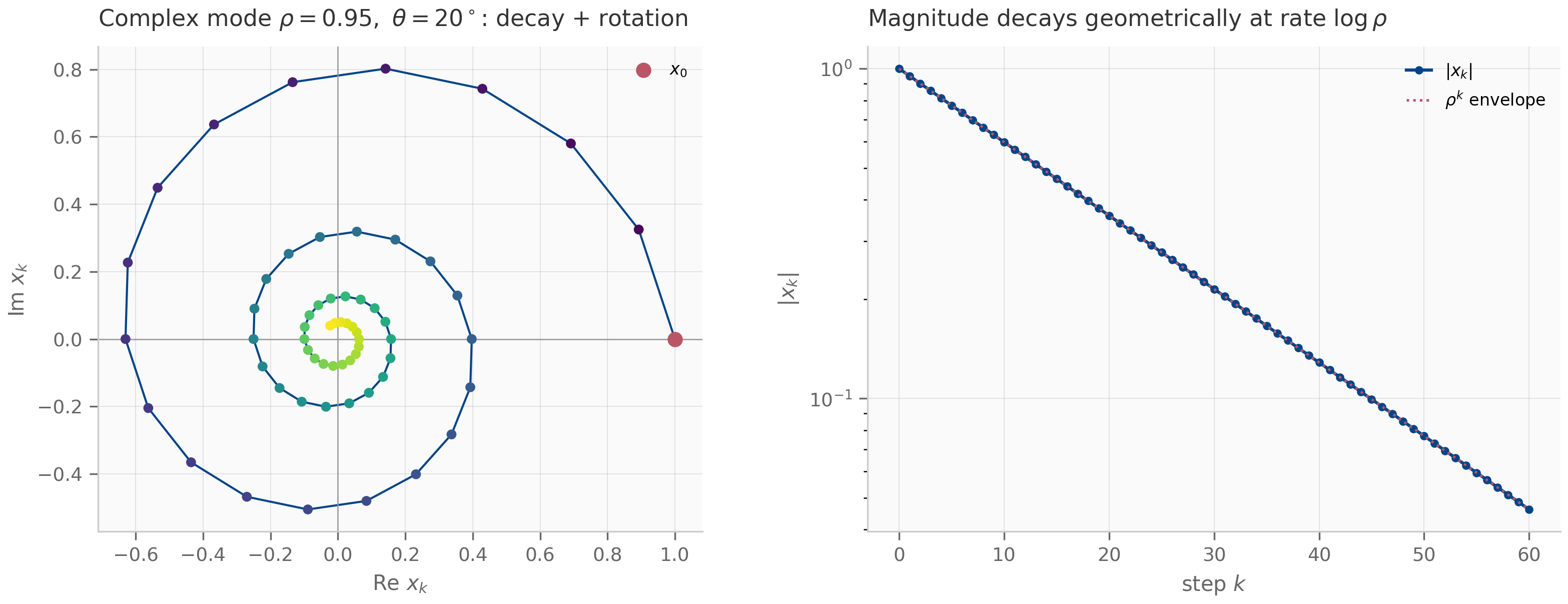
The magnitude decays at rate per unit step and the phase advances by : a single head is now a damped oscillator, tracing the logarithmic spiral of Chapters 1-2 rather than a monotone decay. This lets one head represent an oscillatory feature — a frequency — instead of only a timescale.
In production Mamba-3 never stores a complex dtype. It keeps a real state and applies rotary position embeddings (RoPE) — 2-D rotations — to the projections . The justification is the elementary isomorphism between complex multiplication and rotation-scaling.
Representing as the real vector , multiplication by equals applying the scaled rotation . Consequently the complex recurrence and the real 2-D recurrence produce identical trajectories.
The proof is Exercise 10.5 (§10.9). The companion pins the two recurrences equal to under a random complex drive, and confirms the spiral’s decay rate equals exactly — the empirical content of “decay and oscillation in one head.”
10.5 The trapezoidal SSD pass
The second-order stencil must coexist with the SSD machinery of Chapter 9 — the semiseparable matrix that lets the layer run as a parallel matmul or a linear-time scan. It does, because only the injection stencil changes. Unrolling the trapezoidal recurrence with the state-transition operator (the same as Definition 9.2) splits the output into two semiseparable streams that share the one decay : a right-endpoint stream weighting source by , and a left-endpoint stream weighting source by across the strictly-lower triangle. Both reuse the Chapter 9 segment-sum decay; the order-2 upgrade is two cheap masked matmuls in place of one.
The companion verifies that the dense two-stream matmul reproduces the sequential trapezoidal recurrence to (for both real and complex modes), and that the end-to-end output is genuinely second-order — halving the step size cuts the error by a factor of four. The SSD duality of §9.5 survives the integrator upgrade intact: same matrix, two schedules, now order 2.
10.6 MIMO and the production block
Two further Mamba-3 changes sit outside the integrator-and-state story this chapter develops, and we treat them briefly. MIMO rank- state mixing (the input and output projections each gain a rank- dimension) raises decode-time arithmetic intensity at fixed state size and, Mamba-3 reports, also lifts model quality through the added expressivity (a -point average downstream gain over the SISO variant) — but neither effect changes the discretization or stability story. The full production block — SwiGLU gating, QK-normalization, the bias — wraps the layer studied here; those too are orthogonal to the integrator-and-state question, and we point to the reference implementation rather than reproduce them Lahoti et al. (2026) .
What this chapter isolates is the dynamical-systems substance: a selective SSM (Chapter 9) run with a second-order exponential integrator (Chapters 4-5) and a complex state (Chapters 1-2, 8). The open program — whether geometric integrators (Chapter 6) preserve long-horizon phase structure better than the exponential scheme over the learned eigenvalue spectrum — is the discretization stability atlas the C1 pilot builds, and Chapter 17 returns to it.
10.7 What’s next
Mamba-3 kept Chapter 9’s selectivity and changed two things: a second-order exponential-trapezoidal integrator (accuracy in the forcing, stability from the exact exponential) and a complex state (decay and oscillation in one head), realized via RoPE and computed through the trapezoidal SSD pass. This closes the core SSM line — HiPPO (Chapter 7) to LTI S4/S4D/S5 (Chapter 8) to selective Mamba (Chapter 9) to Mamba-3 (here).
Chapter 11 opens the “beyond SSM” part by taking the SSD duality of §9.6 the other way: linear attention and the Hyena long-convolution lineage enter from the attention side of Theorem 9.5, where the structured contractions of these four chapters reappear wearing transformer clothing.
10.8 Exercises
Six problems: three short (inline solutions), three longer (full solutions in §10.9).
Exercise 10.1 (short)
For a complex mode with , , and step , compute and the phase advance of over two steps. Which is the decay timescale and which is the oscillation frequency?
Solution
, so per step and the phase advances per step. Over two steps and the phase advances . The magnitude sets the decay timescale; sets the oscillation frequency. They are independent — that is the point of a complex mode.
Exercise 10.2 (short, code)
Run companions/ch10/jax/discretization.py. Confirm the fitted convergence slopes
are for ZOH and for exp-trapezoidal on the forced system.
Then explain, in one sentence, why the same script reports both schemes at
on the homogeneous system.
Solution
The script prints ZOH slope and exp-trapezoidal slope on the forced mode. On the homogeneous mode the transition is exact for both schemes, so both reproduce to floating-point roundoff and the order difference — which lives entirely in the forcing coefficients — never enters (Theorem 10.1).
Exercise 10.3 (short)
Write the exp-trapezoidal coefficients for , , and . Show that reduces to a first-order shifted ZOH (no current-input term carrying the decay).
Solution
throughout. : , (pure left endpoint). : , (symmetric). : , — only the current input enters, with no decay applied to it, which is a first-order ZOH shifted by one step. The symmetric is the only second-order member.
Exercise 10.4 (theory) — solution in §10.9
Prove Theorem 10.1: for the exponential-trapezoidal scheme has local truncation error on a forced system, and show that on the homogeneous system both ZOH and exp-trapezoidal are exact.
Exercise 10.5 (theory) — solution in §10.9
Prove Theorem 10.3: that a 2-D rotation by on equals multiplication of by , and conclude the complex and real-RoPE recurrences coincide.
Exercise 10.6 (theory) — solution in §10.9
Prove Theorem 10.2: that the exponential schemes are A-stable with on stiff modes, and contrast the bilinear Padé factor, showing as .
10.9 Full solutions to theory exercises
Solution to Exercise 10.4
Write the exact one-step map by variation of constants over :
The transition is reproduced exactly by both schemes, so all error is in the forcing integral. Exp-trapezoidal approximates , with integrand , by the trapezoidal quadrature rule — the endpoint weights of §10.2. The trapezoidal rule on an interval of width has error for some interior ; since is whenever is , the local truncation error is per step, and summing steps over a fixed horizon yields global order 2. For the homogeneous system the forcing integral vanishes identically and exactly for both schemes, regardless of order — there is no forcing term to approximate, so the order distinction disappears.
Solution to Exercise 10.5
Let and write . Then
whose real-vector form is with . Scaling by commutes with the real isomorphism, so multiplication by is on . Applying this at every step of the affine recurrence (the additive drive maps to componentwise, which the isomorphism also preserves) shows the complex recurrence and the real recurrence produce identical trajectories under .
Solution to Exercise 10.6
For the exponential schemes , so . If and then the exponent is negative and for every (A-stability over the whole left half-plane), and as the mode stiffens () we have . For the bilinear scheme with ; writing with , (the left point is closer to , the right to ), so — also A-stable. But as the ratio , so : stiff modes are mapped to the unit circle and ring rather than decaying. This is the qualitative gap the exponential transition closes.
10.10 Companion code
The companions live in companions/ch10/{jax,julia,torch}/. The JAX module covers
the integrator, the complex state, and the trapezoidal SSD pass; the PyTorch module
mirrors the integrator and complex state (cross-framework parity); the Julia module
is the discretization atlas only — the numerical-analysis core — and joins the
Chapter 4-6 Julia family that the C1 pilot’s stability atlas builds on.
The discretization study (order slopes, homogeneous-blindness, stability regions):
PYTHONPATH=. python companions/ch10/jax/discretization.py
julia --project=companions/ch10/julia companions/ch10/julia/discretization.jl
The complex state and RoPE equivalence (the spiral figure):
PYTHONPATH=. python companions/ch10/jax/complex_state.pyThe trapezoidal SSD pass (matmul equals the sequential oracle):
PYTHONPATH=. python companions/ch10/jax/trapezoidal_ssd.pyThe PyTorch mirror (integrator and complex state, parity-checked against JAX):
PYTHONPATH=. python companions/ch10/torch/discretization.py
PYTHONPATH=. python companions/ch10/torch/complex_state.py
Run the suites — JAX and Julia in the fast loop, torch separately:
make companion-jax-tests
make companion-julia-tests
make companion-torch-tests