Implicit methods, stiff systems, symplectic integration

6.1 Why explicit methods fail: stiffness

Chapter 5 ended with the Dahlquist barrier: no explicit Runge–Kutta method is A-stable. The barrier matters because of a phenomenon called stiffness — when the dynamics matrix $\statemat$ has eigenvalues with very different magnitudes.

A linear ODE $\dot \statevec = \statemat \statevec$ is stiff if $\statemat$ has at least one eigenvalue with $\operatorname{Re}(\lambda_i) \le -1/T$ for a time-scale $T$ much smaller than the simulation horizon, and the eigenvalue is paired with a long-lived (small-$\abs{\lambda}$) mode that one actually wants to track. Stiffness is therefore relative: a system is stiff with respect to a given horizon and given accuracy goal, not in absolute terms. The Robertson chemical-kinetics problem ($\lambda$‘s spanning ten orders of magnitude) is the canonical textbook example; van der Pol at parameter $\mu \gg 1$ is a popular ML-adjacent stand-in because it generates a nonlinear oscillation whose slow and fast phases differ by $\mu$.

For an explicit method, the step size is bounded by the fastest eigenvalue: $\stepsize \lesssim 2/\abs{\lambda_{\max}}$ (forward Euler) or some other small constant times $1/\abs{\lambda_{\max}}$ (RK4). If the slow eigenvalue we want to track is $\abs{\lambda_{\min}}$, the integrator takes $\abs{\lambda_{\max}}/\abs{\lambda_{\min}}$ times more steps than the slow time scale would suggest. For Robertson this ratio is $10^{10}$. The simulation never finishes.

For an SSM, stiffness arises naturally for input-dependent dynamics. Mamba’s selective scan generates an effective $\statemat(u_t)$ at each token; for inputs that produce eigenvalues with very different magnitudes, the time-discretized recurrence is solving a stiff problem at each step. If the discretization is not A-stable, the recurrence either blows up or requires a step size $\stepsize \ll 1$ — at which point you are running the model in an absurd regime. This is the structural reason Mamba-3 switched to exponential-trapezoidal (§4.5), which is A-stable in $\statemat$ but explicit in $u$.

6.2 Implicit methods: backward Euler, BDF, DIRK

The fix for stiffness is to abandon explicit methods. Backward Euler is the simplest implicit method:

Solving for $\statevec_{k+1}$ requires either a linear solve (for linear $f$) or a Newton iteration (for nonlinear $f$). The pay-off is the stability function

which has $\abs{\stabfn_{\text{BE}}(z)} \le 1$ for every $z$ with $\operatorname{Re}(z) \le 0$ — backward Euler is A-stable. It is also L-stable: $\stabfn_{\text{BE}}(z) \to 0$ as $\operatorname{Re}(z) \to -\infty$, so fast modes get damped aggressively as desired on stiff problems.

The proof is one line each: $\abs{1 - z}^2 = (1 - \operatorname{Re}(z))^2 + \operatorname{Im}(z)^2 \ge 1$ when $\operatorname{Re}(z) \le 0$, giving $\abs{\stabfn(z)} \le 1$. The limit is immediate.

Backward Euler is first-order accurate. Higher-order implicit methods come in several families.

BDF$k$ (Backward Differentiation Formula, $k$th-order) is a multi-step method that approximates $\dot \statevec(t_{k+1})$ by a $k$-point backward difference and equates it to $f(\statevec_{k+1})$. BDF1 = backward Euler; BDF2 is second-order and L-stable; BDF$k$ for $k = 3, \ldots, 6$ are conditionally stable but widely used in stiff ODE codes. BDF7 and higher are not zero-stable (the characteristic root condition fails), so they are unusable. The order limit is the second Dahlquist barrier, a structural fact about multi-step methods that we will state without proof: no $A$-stable linear multi-step method has order higher than 2.

Diagonally implicit RK (DIRK) sits between explicit RK and fully implicit RK. The $A$ matrix is lower triangular with non-zero diagonal, so each stage requires solving an independent nonlinear system (cheaper than the coupled system of fully implicit RK, but more expensive than the trivial explicit evaluations). Singly-DIRK (SDIRK) further constrains all diagonal entries to be equal, so the Newton Jacobian factorizes once per step. The Crank–Nicolson (trapezoidal) scheme is a 2-stage ESDIRK of order 2 — its explicit first stage and unequal diagonals place it just outside the strict SDIRK class.

Fully implicit RK — the most expensive family — includes Gauss–Legendre methods, which we will return to in §6.5 as the optimal symplectic methods.

The computational trade-off for implicit methods: each step costs $O(N^3)$ (linear solve for the Jacobian factor) or $O(\text{iterations} \cdot N^2)$ (Newton iteration for nonlinear $f$). For SSMs with $N = 16, 64$ this is acceptable; for $N$ in the thousands it begins to dominate. The Chapter 4 exponential-trapezoidal scheme has the same A-stability as backward Euler but only costs one matrix-exponential per timestep (vs one Newton solve), and the matrix exponential of a low-rank or diagonalized $\statemat$ is cheap. Mamba-3’s specific tactical advantage over a backward-Euler implementation comes down to this cost asymmetry.

6.3 Exponential integrators revisited

The exp-trapezoidal scheme of §4.5 is the simplest member of the exponential integrator family. Recall the general idea: given $\dot \statevec = \statemat \statevec + \inputmat u(t)$, treat the linear part exactly via $e^{\statemat \stepsize}$ and approximate only the forcing integral. The $\varphi$-function family $\varphi_k(z) = (e^z - \sum_{j=0}^{k-1} z^j/j!)/z^k$ provides building blocks for arbitrarily high order.

Three commonly used schemes:

• exp-Euler: $\statevec_{k+1} = e^{\statemat \stepsize} \statevec_k + \stepsize \varphi_1(\statemat \stepsize) \inputmat u_k$. Treats the input as piecewise constant (like ZOH); first-order for forced systems, exact on autonomous problems.
• exp-midpoint: uses the input midpoint instead of $u_k$; second-order for symmetric input perturbations.
• exp-trapezoidal (§4.5): linear interpolation of the input; second-order for $C^1$ inputs.
• ETDRK4 Hochbruck & Ostermann (2010) : a four-stage exponential RK method that achieves fourth order. The Mamba-3 paper Lahoti et al. (2026) does not (yet) use ETDRK4; its second-order exp-trapezoidal is the empirical sweet spot.

All exponential integrators inherit A-stability from $e^{\statemat \stepsize}$. They sidestep the Dahlquist barrier because their stability function is not a polynomial — it is $e^z$ times a rational-in-$z$ correction factor — and the polynomial constraint of explicit RK methods does not apply.

The implementation cost: one matrix exponential plus one or two $\varphi$-function evaluations per step. For a low-rank $\statemat$ (which selective SSMs typically have, since the structured-$\statemat$ pattern of Chapter 7 carries forward), the matrix exponential is cheap. For dense general $\statemat$ exponentials cost $O(N^3)$ via Padé / scaling-and-squaring, the same as a Newton solve — so the choice between exp-trap and backward Euler often comes down to whether you want autonomous-exactness (exp-trap wins) or L-stability damping of high-frequency modes (backward Euler wins).

6.4 Hamiltonian mechanics, energy conservation, and the symplectic structure

The remainder of this chapter introduces the language of Hamiltonian systems and symplectic integration. This is where the direct-transfer hook from continuum mechanics applies most cleanly. The exposition is brief and standalone; for the full theory see Hairer–Lubich–Wanner Hairer et al. (2006) , Chapter VI.

A Hamiltonian system on phase space $(q, p) \in \R^n \times \R^n$ is governed by a scalar function $\hamilton(q, p)$ — the Hamiltonian, intended to represent total energy — through Hamilton’s equations:

The canonical example is the harmonic oscillator $\hamilton(q, p) = \tfrac{1}{2}(p^2 + \omega^2 q^2)$, giving $\dot q = p$, $\dot p = -\omega^2 q$. The pendulum is $\hamilton(q, p) = \tfrac{1}{2} p^2 - \cos(q)$; vortex-dynamics flows are higher-dimensional but structurally identical.

Three properties make Hamiltonian systems geometrically special.

Energy conservation. For a $C^1$ Hamiltonian, along any trajectory $(q(t), p(t))$, $\frac{d}{dt} \hamilton(q(t), p(t)) = \frac{\partial \hamilton}{\partial q} \dot q + \frac{\partial \hamilton}{\partial p} \dot p = \frac{\partial \hamilton}{\partial q} \frac{\partial \hamilton}{\partial p} - \frac{\partial \hamilton}{\partial p} \frac{\partial \hamilton}{\partial q} = 0$. The Hamiltonian is a constant of motion.

Phase-space volume preservation (Liouville’s theorem). The flow $\Phi_t : (q_0, p_0) \mapsto (q(t), p(t))$ has Jacobian determinant 1 everywhere: $\det \nabla \Phi_t \equiv 1$. Volumes in phase space are preserved exactly under the dynamics.

Symplectic structure. Define the symplectic 2-form $\symform = \sum_i dq_i \wedge dp_i$. The flow $\Phi_t$ is a symplectic transformation: it preserves $\symform$ in the sense that $\Phi_t^* \symform = \symform$ where $\Phi_t^*$ denotes the pullback. Symplecticity is a strict refinement of volume preservation — every symplectic transformation is volume-preserving, but not vice versa.

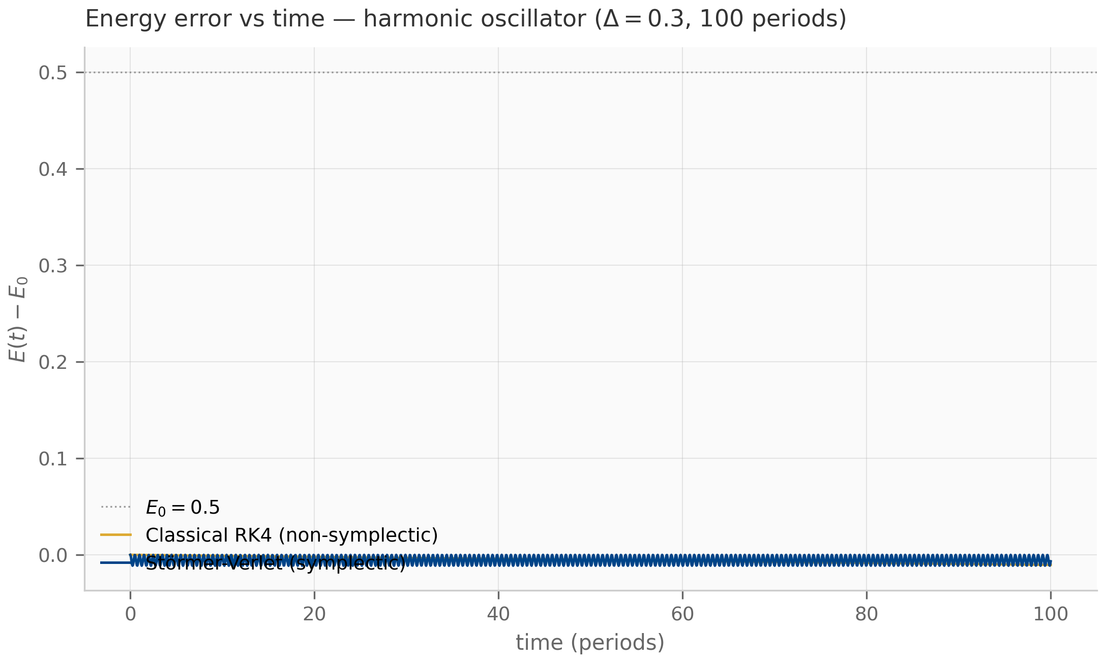
The reason these properties matter for numerics is that standard order-optimized integrators destroy them. A fourth-order RK method simulates the harmonic oscillator with $O(\stepsize^4)$ global error in the state — but it does not exactly preserve energy. The energy error accumulates monotonically (one-sided, not oscillating around the initial value), producing a linear-in-time energy drift whose rate depends on the problem nonlinearity and step size.

On the linear harmonic oscillator at small $\stepsize$ the rate is impressively small: RK4’s stability function $R(z) = \sum_{j=0}^{4} z^j/j!$ is not time-symmetric (a symmetric method satisfies $R(z)R(-z) = 1$; RK4 instead gives $1 + z^6/72 + \cdots$), so on the imaginary axis $\abs{R(i\theta)}^2 = 1 - \theta^6/72 + \cdots < 1$ and the energy is very slightly, monotonically damped — the slow negative drift the symplectic_demo.py companion exhibits. It remains monotonic in a way symplectic methods are not.

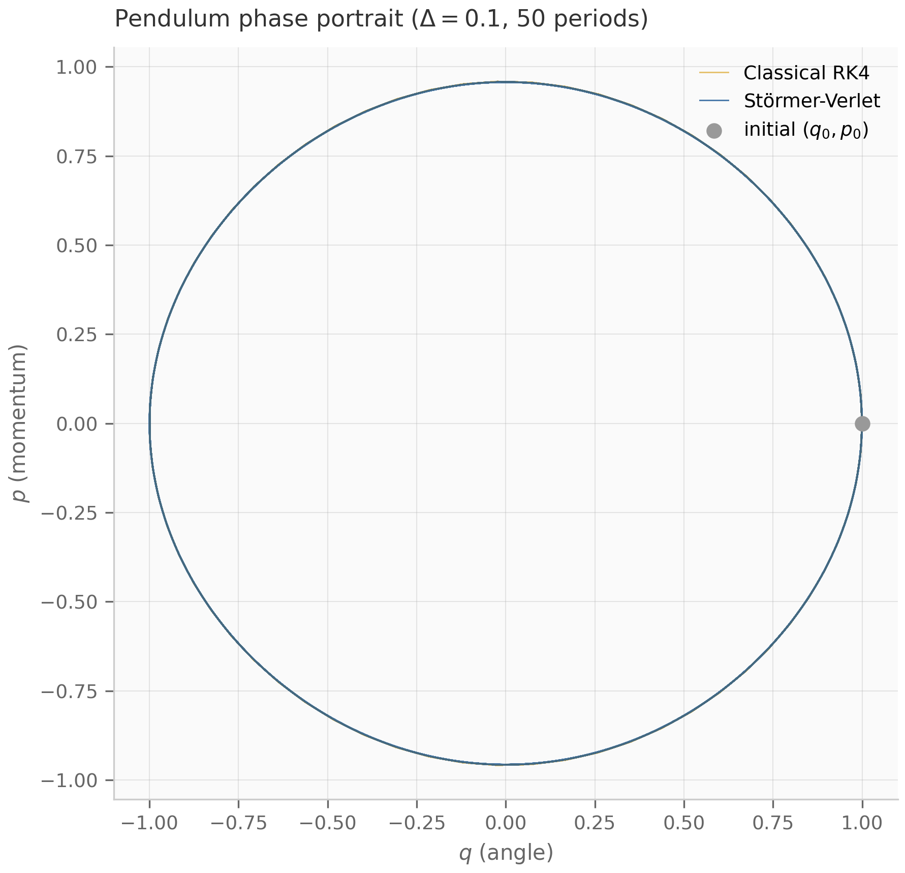
As $\stepsize$ grows or the problem becomes nonlinear the rate becomes visible: at $\stepsize \approx 0.3$ over 1000 periods of the pendulum, RK4 drifts by $\sim 10^{-2}$ in energy and noticeably distorts the orbit; at large enough $\stepsize$ the orbit eventually escapes the bound regime. On a Kepler problem the analogous failure mode is eventual ejection or capture of the orbiting body. These are not numerical instabilities in the Chapter 5 sense — the method is A-stable for the small-amplitude regime — they are geometric errors: the wrong qualitative dynamics, made visible at sufficient horizon.

6.5 Symplectic integrators

A symplectic integrator is a numerical map $\Psi_\stepsize : (q, p) \mapsto (q', p')$ that preserves the symplectic 2-form: $\Psi_\stepsize^* \symform = \symform$. Symplectic integrators do not, in general, preserve $\hamilton$ exactly — but they preserve a nearby modified Hamiltonian $\widetilde \hamilton = \hamilton + O(\stepsize^p)$ for a $p$-th order symplectic method. As a consequence, the energy $\hamilton(q_k, p_k)$ along the discrete trajectory oscillates within a bounded band of width $O(\stepsize^p)$ around its initial value — not drifting linearly with $t$, but staying near a level set of $\widetilde \hamilton$. This is the backward error analysis of geometric integrators, and it is the practical reason symplectic methods are mandatory for long-horizon Hamiltonian simulations.

Three canonical schemes.

Symplectic Euler (1st order). For a separable Hamiltonian $\hamilton(q, p) = T(p) + V(q)$:

Update momentum first using position-derived force; then update position using the updated momentum. The asymmetry — using $p_{k+1}$ in the second step rather than $p_k$ — is what makes the scheme symplectic. A symmetric version updates $q$ first, then $p$; both are valid.

Störmer–Verlet (2nd order, symmetric). A symmetric version of symplectic Euler that does a half-step in momentum, full step in position, half-step in momentum:

This is the algorithm used in essentially every molecular-dynamics simulation. Second-order accurate, symplectic, time-reversible (the same algorithm run with $-\stepsize$ exactly reverses the trajectory). The energy error is bounded by $O(\stepsize^2)$ over arbitrarily long horizons.

Gauss–Legendre IRK (order $2s$, A-stable, symplectic). The $s$-stage Gauss–Legendre Runge–Kutta method has nodes at the Gauss–Legendre quadrature points and is the unique $s$-stage implicit RK method of order $2s$ (the maximum attainable for $s$ stages). The 1-stage method is the implicit midpoint rule (order 2, symplectic, A-stable). The 2-stage method is order 4. Gauss–Legendre IRK is the unique family that is simultaneously A-stable, symplectic, and of optimal order — making it the gold standard for high-accuracy long-horizon Hamiltonian simulation Hairer et al. (2006) .

The proof — Hairer–Lubich–Wanner Chapter IX — uses backward error analysis to expand the modified Hamiltonian as an asymptotic series in $\stepsize$ and shows the series can be truncated with controlled remainder. The takeaway for practice: a $p$-th order symplectic integrator is exponentially better than a $p$-th order non-symplectic one on Hamiltonian problems, even though the local truncation error of both is $O(\stepsize^{p+1})$. Local error is misleading for long-horizon problems; geometric structure is what matters.

6.6 Toward selective SSMs as Hamiltonian flows

The C1 niche pilot proposes the following research program. The hidden-state dynamics of a selective SSM can sometimes be written as a Hamiltonian flow on the hidden-state manifold; when they can, applying a symplectic integrator should reduce long-horizon error in a way that order-optimized integrators cannot match. The first step is to characterize when this Hamiltonian structure exists.

For a linear-time-invariant SSM $\dot \statevec = \statemat \statevec$, the dynamics are Hamiltonian iff there exists a symmetric positive-definite $P$ such that $\statemat^\top P + P \statemat = 0$. Equivalently, $\statemat$ is similar (via $P^{1/2}$) to a skew-symmetric matrix. The quadratic Hamiltonian is then $\hamilton(\statevec) = \tfrac{1}{2} \statevec^\top P \statevec$, and the symplectic 2-form is $\symform = P^{-1}$ (in the standard symplectic-flat coordinates). For HiPPO-LegS the eigenvalues are all real-negative, not purely imaginary, so HiPPO-LegS dynamics are dissipative, not Hamiltonian. Symplectic methods do not apply. This is consistent with the empirical observation that ZOH and bilinear discretizations of HiPPO-LegS perform well — dissipation handles the long-horizon stability story.

For a selective SSM with input-dependent $\statemat(u)$, the relevant question becomes: does $\statemat(u)$ have a Hamiltonian decomposition for some range of inputs, even if not for all? The C1 pilot’s empirical hypothesis is that during certain training phases the learned $\statemat(u)$ matrices drift toward eigenvalue spectra that are closer to purely imaginary than to the LHP, and that this drift is associated with the long-horizon recall artifacts observed in Mamba’s failure modes Halloran et al. (2025) . If this hypothesis holds, then symplectic discretization of selective SSMs should reduce those artifacts. The Chapter 17 pilot integration develops this thread; this chapter has supplied the necessary integration-theory vocabulary.

6.7 What’s next

This chapter completes the foundations layer of the book (Part I). The next part — Chapters 7–10 — introduces structured SSMs (S4, S4D, S5, Mamba-1/2, Mamba-3) as discretizations of the continuous systems developed here. Chapter 7 sets up HiPPO theory; Chapter 8 derives the S4 / S4D / S5 architectures (and sorts out which discretization each paper actually used); Chapter 9 introduces selective scans (Mamba-1/2); Chapter 10 brings the exp-trapezoidal scheme of §4.5 to its home in Mamba-3.

The C1 pilot integration in Chapter 17 returns to this chapter’s symplectic story, applying the modified-Hamiltonian framework to learned selective dynamics. Readers focused on the SSM applications can skip to Chapter 7 now and consult §6.5–§6.6 when the symplectic discussion comes back.

6.8 Exercises

Six problems. Short/numerical (6.1–6.3) have inline collapsible solutions; long/proof exercises (6.4–6.6) have full worked solutions in §6.9.

Exercise 6.1 (computation)

Verify that backward Euler’s stability function is $\stabfn_{\text{BE}}(z) = 1/(1-z)$ by directly applying the scheme to the test problem $\dot y = \lambda y$ and solving for $y_{k+1}$.

Exercise 6.2 (computation)

For the harmonic oscillator $\dot q = p$, $\dot p = -q$ (so $\hamilton = (p^2 + q^2)/2$), compute one step of symplectic Euler (“p first” variant) starting from $(q_0, p_0) = (1, 0)$ at $\stepsize = 0.1$. What are $(q_1, p_1)$, and what is $\hamilton(q_1, p_1)$?

Exercise 6.3 (computation + code)

Run companions/ch06/jax/symplectic_demo.py. Verify that classical RK4 produces linear-in-time energy drift on the harmonic oscillator while Störmer–Verlet’s energy stays in a bounded band. What is the drift rate (energy per period) of RK4 at $\stepsize = 0.05$?

Exercise 6.4 (theory) — solution in §6.9

Prove the L-stability of backward Euler (Proposition 6.1): $\abs{\stabfn_{\text{BE}}(z)} \le 1$ for $\operatorname{Re}(z) \le 0$, and $\stabfn_{\text{BE}}(z) \to 0$ as $\operatorname{Re}(z) \to -\infty$.

Exercise 6.5 (theory) — solution in §6.9

Show that symplectic Euler is symplectic. That is, prove that the Jacobian $\partial(q_{k+1}, p_{k+1})/\partial(q_k, p_k)$ has determinant exactly 1 for the harmonic oscillator. (Then note: for separable Hamiltonians, the same argument applies via the chain rule.)

Exercise 6.6 (theory) — solution in §6.9

Show that for a linear-time-invariant ODE $\dot \statevec = \statemat \statevec$ with $\statemat$ skew-symmetric ($\statemat^\top = -\statemat$), the function $\hamilton(\statevec) = \tfrac{1}{2} \statevec^\top \statevec$ is a constant of motion. Use this to give a sufficient condition (in terms of $\statemat$ only) for an SSM to be Hamiltonian.

6.9 Full solutions to theory exercises

Solution to Exercise 6.4

Write $z = -r + i\omega$ with $r \ge 0$. Then $\abs{1 - z}^2 = (1 + r)^2 + \omega^2$. Since $r \ge 0$, $(1 + r)^2 \ge 1$, so $\abs{1 - z}^2 \ge 1$. Therefore $\abs{\stabfn_{\text{BE}}(z)} = 1/\abs{1 - z} \le 1$. ∎

For the L-stability limit: as $r \to \infty$ with $\omega$ bounded, $\abs{1 - z}^2 = (1 + r)^2 + \omega^2 \to \infty$, so $\stabfn_{\text{BE}}(z) \to 0$. ∎

Solution to Exercise 6.5

For the harmonic oscillator $\dot q = p$, $\dot p = -q$, symplectic Euler ($p$ first) gives

The Jacobian is

The determinant: $\det J = (1 - \stepsize^2)(1) - \stepsize \cdot (-\stepsize) = 1 - \stepsize^2 + \stepsize^2 = 1$. ∎

So the discrete map preserves the symplectic 2-form $dq \wedge dp$ exactly. This is the algebraic content of “symplectic Euler is symplectic” — the determinant being exactly $1$, not $1 + O(\stepsize^p)$.

For a general separable Hamiltonian $\hamilton = T(p) + V(q)$, symplectic Euler gives $p_{k+1} = p_k - \stepsize V'(q_k)$ and $q_{k+1} = q_k + \stepsize T'(p_{k+1})$. The Jacobian factorizes as

each of which has determinant 1 (lower- and upper-triangular with 1s on the diagonal). The product determinant is therefore 1. ∎

This “shear-decomposition” argument generalizes to all symplectic integrators that update $q$ and $p$ in alternating steps: each individual sub-step is a shear, with unit determinant. Verlet, leapfrog, Yoshida composition methods — all are products of unit-determinant shears.

Solution to Exercise 6.6

For $\dot \statevec = \statemat \statevec$ with $\statemat^\top = -\statemat$, compute

since $\statemat^\top + \statemat = 0$ by skew-symmetry. So $\hamilton(\statevec(t)) \equiv \hamilton(\statevec_0)$ — the squared norm is exactly preserved. ∎

Sufficient condition for an SSM to be Hamiltonian. Any SSM whose continuous dynamics matrix $\statemat$ is skew-symmetric is Hamiltonian with Hamiltonian $\hamilton(\statevec) = \tfrac{1}{2} \statevec^\top \statevec$. The eigenvalues of a real skew-symmetric matrix are purely imaginary (or zero), so this regime is exactly the purely oscillatory corner of the SSM landscape — the opposite of the LHP-stable corner where HiPPO and S4 live. A more general sufficient condition: $\statemat$ has a Hamiltonian structure (in the matrix-Lie-algebra sense) — equivalently, there exists a symmetric positive-definite $P$ with $\statemat^\top P + P \statemat = 0$. The C1 pilot’s empirical project is to identify selective-SSM regimes where this condition holds approximately, and to apply symplectic discretization there.

6.10 Companion code

Two JAX companions, two PyTorch companions, and two Julia companions for Chapter 6.

JAX (companions/ch06/jax/):

• stiff_demo.py — van der Pol oscillator at $\mu = 10$ (mildly stiff); compares explicit RK4 (blows up at large $\stepsize$) against backward Euler (stable at every $\stepsize$); emits stiff_blowup.png.
• symplectic_demo.py — harmonic oscillator + pendulum; runs classical RK4 vs Störmer–Verlet over 100 periods; emits energy_drift.png and phase_portrait.png.

Julia (companions/ch06/julia/):

• implicit_methods.jl — backward Euler, BDF2, and DIRK from-scratch implementations on a stiff test problem; uses only LinearAlgebra + Printf.
• symplectic_methods.jl — symplectic Euler, Störmer–Verlet, and the 2-stage Gauss–Legendre IRK method on a Hamiltonian test; emits empirical order-of-accuracy table.
• Project.toml / Manifest.toml.

PyTorch (companions/ch06/torch/):

• stiff_demo.py — the van der Pol RHS/Jacobian with RK4 and backward-Euler steppers (compute-only; the JAX companion produces the figure).
• symplectic_demo.py — the RK4 and Störmer–Verlet steppers on the harmonic oscillator and pendulum.
• tests/ — cross-framework parity: the torch trajectories and energy-drift quantities equal their JAX counterparts to within $10^{-9}$ (float64).

To run from the repo root:

# JAX
PYTHONPATH=. python companions/ch06/jax/stiff_demo.py
PYTHONPATH=. python companions/ch06/jax/symplectic_demo.py

# PyTorch (needs the .venv [torch] extra; parity only, no figures)
PYTHONPATH=. python companions/ch06/torch/stiff_demo.py
PYTHONPATH=. python companions/ch06/torch/symplectic_demo.py

# Julia (lightweight — no DifferentialEquations.jl dependency)
julia --project=companions/ch06/julia companions/ch06/julia/implicit_methods.jl
julia --project=companions/ch06/julia companions/ch06/julia/symplectic_methods.jl

All figures emit to public/figures/ch06/.