Empirical methodology: benchmark protocols and evaluation

16.1 The measurement problem

This book has spent fifteen chapters arguing that sequence architectures are points in one design space, not rival species: a selective SSM is a masked linear-attention computation (Theorem 9.5), an additive state holds only as many associations as its rank allows (Proposition 11.4), smarter write rules buy capacity at the price of a stability analysis (Theorem 12.4), and a hybrid is a budget split between exact local computation and compressed carried state (Proposition 14.2). Every one of those claims ends in an empirical question: given two points in the design space, how do you tell which is better, and for what? Chapter 12 promised that the comparisons across its lineage would be made honest here; Chapter 14 handed over a benchmark seed and deferred its protocol. This chapter pays both debts.

The premise is that a benchmark is a measurement instrument, and deserves the same scrutiny as any other instrument: what quantity does it respond to, over what operating range, with what noise floor? The lens chapters tell us what the quantities are. A finite state has a capacity — so there must be a probe that loads it past capacity. Real streams have timescales — so there must be a task whose slow variable a window cannot see and whose decay rate a state must match. Exactness has a range — so there must be a stress that separates content the model must retrieve from content it may forget. And every one of these costs resources — cache, state, throughput — that the comparison must hold fixed or report. None of this is hypothetical: the synthetic-probe methodology of MAD Poli et al. (2024) and Zoology Arora et al. (2024) exists precisely because small tasks chosen this way predicted which architectures were worth pretraining.

What the lens does not supply is automatic validity. A probe can be solvable by machinery unrelated to its advertised quantity; a length stress can fail to stress anything; an evaluation can launder noise into a ranking. Each failure mode appears below with an exact, companion-checked example — including one we built by accident and kept as teaching material.

The chapter is organized as an evaluation stack with four tiers, numbered cheap to expensive: Tier 1 — mechanism probes, synthetic tasks isolating one capability, minutes to run (§16.2); Tier 2 — synthetic long-context stress with controlled length and timescale dials (§§16.4–16.5); Tier 3 — natural long-document suites, realistic but noisy (§16.4); Tier 4 — language-model quality and systems efficiency, the expensive anchor (§16.6). The statistics of §16.3 apply at every tier, and matter most where evaluation is noisiest.

16.2 Synthetic probes and the discriminative regime

A mechanism probe earns its keep by isolating one capability so cleanly that failure has a unique explanation. The Tier-1 canon, by target capability:

• associative recall — multi-query associative recall (MQAR): store key–value pairs, answer queries about them. The probe Zoology built, and the one Chapter 11 used to measure the capacity wall Arora et al. (2024) .
• in-context pattern completion — the induction-head task: attend to the previous occurrence of the current token and copy its successor Olsson et al. (2022) .
• selective copying — copy designated tokens while ignoring filler; the probe that motivated input-dependent selectivity Gu & Dao (2024) .
• string copying at length — reproduce an input verbatim. Copying a length-$n$ string means carrying $n$ tokens of information, so a fixed $d$-dimensional state must fail once $n$ outruns its capacity while the attention cache grows with the input by construction; Jelassi et al. (2024) prove the separation in its strongest form — a two-layer transformer can copy strings of exponential length while fixed-state models are fundamentally limited by their state — which is the empirical face of Chapter 3’s Krylov-dimension reading of the recurrence’s expressive ceiling, and redeems that chapter’s promise here. The impossibility side of the story (what else fixed state provably cannot do) is Chapter 15’s file.
• composite suites — MAD’s six-task battery, used as a cheap screen whose scores rank-correlate with scaling behaviour Poli et al. (2024) .

Zoology’s central finding is that the language-model quality gap between efficient architectures and attention traces to associative-recall capability specifically — which is what made MQAR this tier’s anchor probe, and the reason the tier exists.

The companion builds the tokenized MQAR object end to end: episodes $[k_1, v_1, \dots, k_N, v_N, \text{(distractors)}, \text{(gap)}, q_1, \dots, q_N]$ with disjoint key/value/filler alphabets, distinct keys, and every target key queried exactly once; ground truth defined by an independent scan oracle; and a family of exact readers standing in for architectures, in the same no-training discipline as §14.6 — each reader is an information restriction, so every curve below is a computation rather than an optimization outcome. The induction reader (exact-match attention reading the successor token — the Olsson et al. (2022) circuit as an analytic object) answers correctly at every load. The outer-product reader (the Proposition 11.4 mechanism on token embeddings) degrades smoothly past its dimension. And the slot reader — a ring buffer keeping the last $d$ pairs, abstaining on evicted keys — is the exact-capacity idealization, with accuracy exactly $\min(1, d/N)$ at load $N$: the caricature of a fixed-size state with a hard edge.

The slot reader is deliberately simple, because simplicity is what makes the section’s design principle a theorem rather than a heuristic:

The proof is four lines (Exercise 16.1 walks an instance). Exactly $\min(N, d)$ of the $N$ queried keys remain in a last-$d$ buffer, and abstention makes accidental correctness impossible, giving the accuracy formula with equality; the three regimes of $G$ follow by cases on $N \lessgtr d_1, d_2$, with monotonicity on $(d_1, d_2]$ because $1 - d_1/N$ increases in $N$. The companion checks the accuracy identity at rtol=0 — not approximately, exactly — and the gap curve below peaks at $0.75 = 1 - 16/64$ at $N = 64$, is identically zero through $N = 16$, and has fallen to $0.0938$ by $N = 512$.

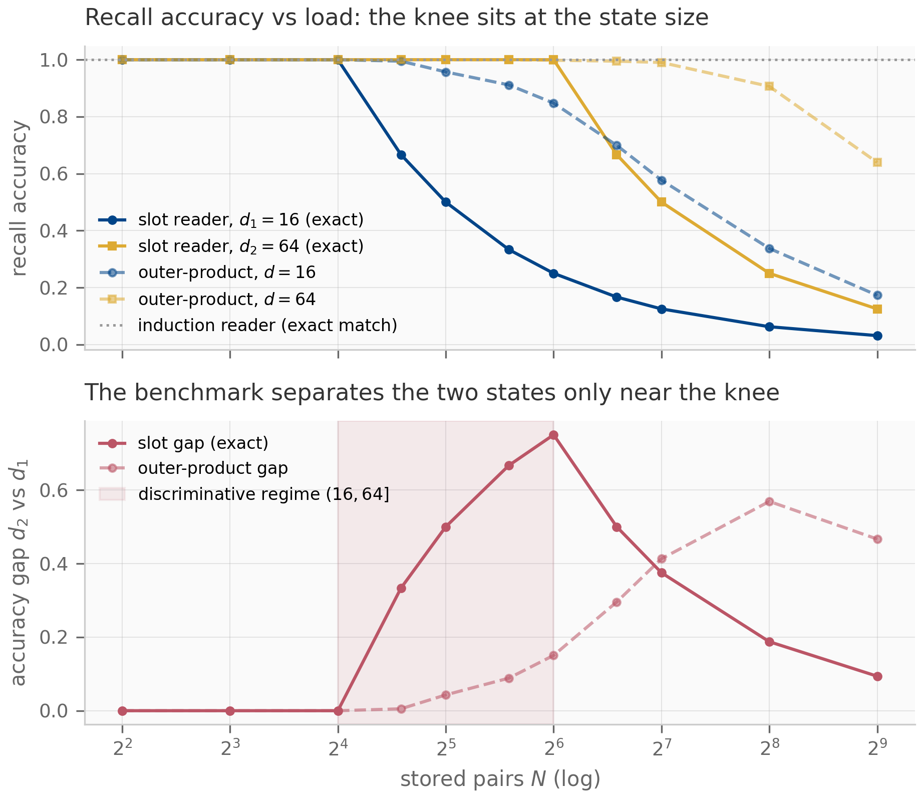
Two readings of the figure, one per direction of generalization. Soft readers shift, but do not escape, the principle. The outer-product reader’s gap peaks at $N = 256$, not $64$: argmax decoding over value embeddings tolerates interference below a threshold, so the effective capacity sits above the raw dimension — but the gap still vanishes at small loads and still decays at large ones, and only the knee’s location moved. Calibrate the load to the mechanism actually under test, not to the nominal state size. The principle is Chapter 14’s lesson in a second coordinate. There, a two-timescale task separates window from carried state only when $w \ll \tau_{\mathrm{id}} \ll 1/\varepsilon$; here, a recall task separates two capacities only when $d_1 < N \lesssim d_2$. Both are instances of one rule: report the dial that places the task in its discriminative regime ($\bar{\imath}$ there, $N$ here) as a first-class task parameter — a benchmark score without its dial setting is a number without units. The copying probe obeys the same rule: its dial is string length against state capacity, which is exactly why Jelassi et al. (2024) sweep length and why a copying score quoted at one length says little.

16.3 The statistics of honest comparison

Tier-1 probes are nearly noise-free — exact readers, exact oracles. Every tier above them is not, and two statistical failure modes account for a large share of unreproducible architecture comparisons. Both have exact antidotes, and both antidotes are cheap.

Pairing. Two predictors evaluated on the same items produce correlated scores: the items hard for one are mostly hard for the other. The honest uncertainty for a mean difference subtracts that shared difficulty; treating the two score sets as independent samples leaves it in.

The proof is the variance of a difference of correlated means (Exercise 16.4). The companion’s demonstration uses the §16.5 reference stream: the window-8 and composite predictors differ by $0.0145$ nats of per-token log loss over $n = 8063$ shared positions, with per-item correlation $0.9867$. The paired standard error is $0.00158$; the unpaired formula gives $0.01370$ — $8.66\times$ larger. The same measured difference is a $z = 9.2$ result with the correct statistic and an unpublishable $z = 1.1$ with the wrong one. Pairing is not a refinement; it decides whether the experiment worked.

Selection. The second failure mode is quieter: evaluate $k$ variants — seeds, sweeps, ablation cells — and report the best. If the variants are equally good, the reported number still exceeds the truth by the expected maximum of $k$ noise draws.

The proof is five lines with the moment generating function (Exercise 16.5). Measured on Gaussian draws, the expectation reaches $1.75\sigma$ at $k = 16$ and $2.34\sigma$ at $k = 64$ against bounds of $2.35\sigma$ and $2.88\sigma$ — the bound is conservative but the growth is real:

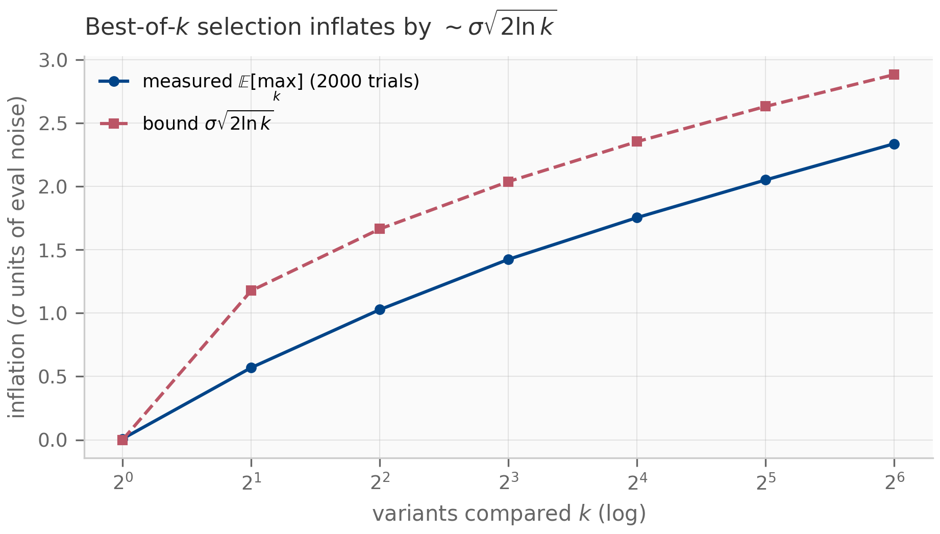
And measured in the wild: scoring $16$ embedding seeds of the same outer-product reader (identical true accuracy by symmetry) on the same $64$-episode battery, the best seed beats the across-seed mean by $+0.0051$ accuracy — against a predicted $1.75 \times 0.0028 = 0.0049$ from the measured seed spread $\sigma = 0.0028$. The theory prices the malpractice to within a rounding error.

The protocol consequences fit in three rules. Pair everything pairable: evaluate all variants on identical items and report paired SEs (per-token losses pair naturally; per-episode accuracies pair across shared episodes). Freeze the suite before the sweep: a task set adjusted after seeing results is a selection mechanism, and inherits the $\sqrt{2 \ln k}$ tax without disclosing its $k$. Report the sweep, not its maximum: best-of-$k$ is legitimate model selection exactly when the selected model is re-scored on data the selection never touched — the held-out discipline every probe in this chapter applies, down to the ridge probe of §16.5 fitting on the first half of a stream and scoring on the second.

16.4 Long-context evaluation and length-robustness metrics

Tier 2 asks the question the lens cares most about: does the mechanism hold at separations it was not tuned on? The field’s instruments here have a cautionary history worth one paragraph. Long Range Arena Tay et al. (2021) defined the long-context battlefield of 2020–2022 — six classification tasks at lengths $1$–$16$K, culminating in Path-X — and S4 famously broke it open, solving Path-X for the first time ( Gu et al. (2022) ; Chapter 8’s kernel machinery is why it could).

The current Tier-2/3 workhorses ask retrieval questions directly. Needle-in-a-haystack stress plants target content at controlled depths in long filler and queries it; RULER Hsieh et al. (2024) systematizes this with multi-key, multi-value, and aggregation variants at controlled lengths, and reports large gaps between claimed and effective context across model families — the single most protocol-shaped finding in the long-context literature: a context-window number on a model card is a claim about an instrument’s range, and RULER is the calibration. On the natural-document side (Tier 3), SCROLLS Shaham et al. (2022) and LongBench Bai et al. (2024) aggregate QA, summarization, and reasoning over real long documents — high validity, but noisy generative metrics (F1, ROUGE) at modest item counts, which is precisely where §16.3’s paired statistics earn their keep.

What should the synthetic version of length stress look like? The companion answers with a negative control we hit by accident. Take the fading-memory reader — the outer-product state decayed by $\rho$ per token, the cleanest caricature of a fixed-rate forgetting recurrence — and stress it by widening the key-to-query separation with neutral filler. Nothing happens. Exactly nothing: every stored weight rescales by the same $\rho^{g}$, argmax decoding is scale-invariant, and the companion pins prediction-level equality between gap $0$ and gap $512$ at rtol=0. A NIAH-style stress built on blank padding measures nothing about fading memory. What stresses it is fresher competing content: $s$ distractor pairs written after the targets leave the target signal at $\rho^{2s + O(1)}$ against interference that decayed far less. RULER’s multi-key variants embody the same insight (the haystack is made of hay, not vacuum); the companion makes it exact, and the design rule is pad with content, not blanks.

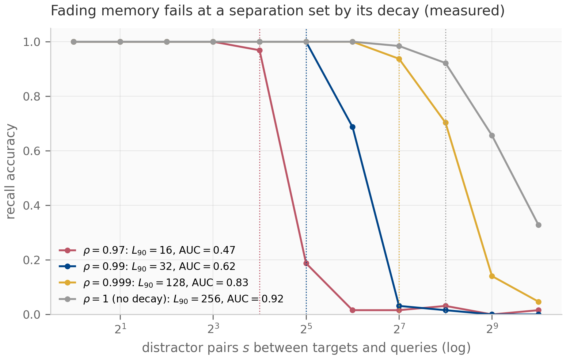
The figure also separates two failure modes the single word “fails at length” conflates: the decayed readers fail by recency (the target faded), the undecayed one by capacity (the buffer filled) — same downward curves, different mechanisms, distinguishable because the generator controls $s$ and $\rho$ independently. That is the Tier-2 advantage over Tier 3 in one picture.

Curves invite single-number summaries, and the long-context literature’s single-number practice is worth formalizing. For a measured accuracy curve $\mathrm{acc}(s)$ over a strictly increasing separation grid $s_1 < \dots < s_m$:

• $L_{90} = \max\{\, s_j : \mathrm{acc}(s_j) \ge 0.9\, \mathrm{acc}(s_1) \,\}$ — the longest separation retaining $90\%$ of short-range accuracy (the range of the instrument, in the calibration sense);
• $\mathrm{AUC} = \int \mathrm{acc}\; d(\log_2 s) \,\big/\, (\log_2 s_m - \log_2 s_1)$ — mean accuracy per octave of separation (trapezoid on the measured grid), rewarding robustness across scales rather than across raw tokens.

Both are implemented and exactness-tested in the companion (hand-constructed curves, rtol=0), and both inherit §16.2’s caveat: a single $L_{90}$ without its grid and task dials is a number without units — report the curve, quote the summary.

16.5 The two-timescale protocol

Chapter 14 shipped pilot B’s task: the two-timescale HMM — slow regime, sticky transition $T(\varepsilon)$, regime-conditioned bigrams with overlap dial $\eta$ — with its exact restriction family, the matched-decay optimality theorem (Theorem 14.4), and the measured design constraint $w \ll \tau_{\mathrm{id}} \ll 1/\varepsilon$ (Figure 14.3). It deferred two things to the protocol: the composite predictor, and the probing method. Both are now in companions/ch16/jax/protocol.py, computed on the same reference instance as Chapter 14’s figures — same constants, same key derivation — so every number here is directly comparable with §14.6’s (the optimal filter’s $1.9289$ nats below is bit-for-bit Chapter 14’s).

The composite restriction. A window-$w$ filter restarted from a uniform prior wastes whatever the past knew; a fixed-decay filter carries the past but applies a possibly mistimed transition at every step. The composite is the natural hybrid idealization: exact Bayes updates (true transition) over the last $w$ tokens, seeded at the window edge with the $\lambda$-decay filter’s posterior — the carried prior a fixed-decay recurrence could actually hand to an attention window. It comes with two machine-checked identities. With a uniform edge prior it is Chapter 14’s window filter (measured difference $0.0$ — two independently written implementations). And with $\lambda = \lambda^\star(\varepsilon)$ it reproduces the full Bayes filter at every window size (measured difference $2.2 \times 10^{-16}$ at $w = 8$): the matched carried prior is the true posterior, exact updates keep it true, and the window adds nothing because nothing was missing — Chapter 14’s matched-decay theorem composing exactly with windowed inference, the idealized version of the matched expansion of §14.2’s lens. Between the identities sits the measurement. At the reference operating point — the carry mistimed at $\lambda^\star(0.2)$ where the truth is $\varepsilon = 0.02$, the same mistiming §14.6 measured — window-8 alone pays $0.0246$ excess nats, the mistimed decay alone pays $0.0512$, and the composite pays $0.0101$ — beating its window part by $0.0145$ nats and its decay part by $0.0411$. A hybrid of two individually mistimed resources beats both, because the window supplies exactness where the carry is stale and the carry supplies memory where the window is blind. That is §14.2’s division of labour as a single measured number.

Why probing is justified — and what it cannot show. Pilot B’s central axis asks where a trained hybrid stores the slow variable, and its method is per-layer probing. Before trusting probes, one should ask what near-optimal prediction actually guarantees. Notation for the answer: $B \in \mathbb{R}^{K \times V \times V}$ stacks the $K$ regime bigram tables over the vocabulary of size $V$, so $B[:, a, :]$ is the $K \times V$ matrix whose $j$-th row is regime $j$‘s next-token distribution given current token $a$. For this task the guarantee is a proposition:

Part (i) is one line (the cross-entropy decomposition; Exercise 16.6), and part (ii) is Pinsker plus norm comparison plus Jensen. The companion checks both numerically: the per-position identity behind (i) holds in closed form to $10^{-12}$ with the realized sample excess matching the mean divergence within Monte-Carlo error, and on the reference instance $\sigma = 0.0402 > 0$, with the regime priors of two different restrictions recovered from their predictive distributions alone — both below $10^{-10}$ in the pinned test, the uniform-restart one to $1.99 \times 10^{-15}$. The honest reading cuts both ways. The proposition justifies the probing program: the slow variable is provably present in any near-optimal predictor, so looking for it is not wishful. It does not say the information sits in any particular layer, that it is linearly decodable from internal activations, or that probe accuracy measures causal use — probing remains correlational, the inversion constant $1/\sigma$ can be large (here $\approx 25$), and locating the information in a trained network is exactly B’s empirical question, not a corollary. Prior art on trained hybrids — e.g. the memory-recall analyses of Lee et al. (2025) — operates under the same caveat.

The probe signature, demonstrated on idealized states. The protocol’s method: extract each candidate state, fit a closed-form ridge probe to the regime labels on the first half of the stream, report held-out argmax accuracy on the second half (the §16.3 discipline; deterministic end to end). Run on each restriction’s internal regime prior — its only carried state — the method produces the disentanglement signature pilot B will look for in trained hybrids:

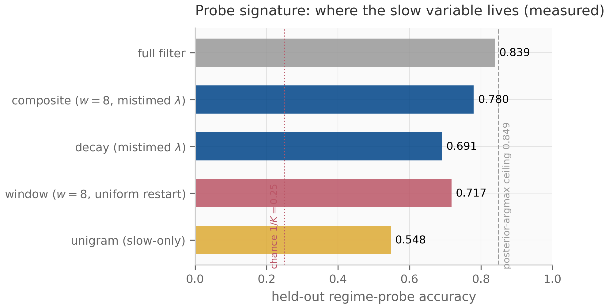
Four measured readings. The full filter’s prior probes at $0.839$, essentially at the ceiling — the exact posterior’s own argmax accuracy, $0.849$, which sits below $1$ because even Bayes stays uncertain on this task at this overlap and switch rate. The composite’s carried prior adds $+0.062$ probe accuracy over the uniform restart — the slow variable demonstrably lives in the carry. The mistimed decay alone probes below the window ($0.691$ vs $0.717$): a sufficiently mistimed memory is worth less than a short exact window even for tracking the slow variable itself — mistiming is not a discount, it is data loss, the probing face of §14.6’s V-shaped cost. And every restriction sits far above chance: this task’s regimes leak into everything, which is why the profile across states, not any single accuracy, is the signature.

The signature slots into pilot B’s reporting scheme of five axes — (A) local capability (short-context LM quality), (B) long-context retrieval, (C) compositional reasoning, (D) fast/slow disentanglement (the signature above — B’s contribution), and (E) systems efficiency — because §14.5’s production lineup showed that hybrids are sold on A+E and differentiated on B — while D is precisely the axis nobody yet measures, which is B’s premise — and a benchmark that collapses the axes into one score reproduces exactly the incommensurability this chapter exists to remove.

The chapter’s protocol contribution ends where B’s empirical work begins, and the boundary is worth stating exactly: everything above is computed on exact filters with known semantics — the protocol mechanics, validated in the only setting where ground truth is available. B applies the same mechanics — same task family, same paired statistics, same probe — to trained attention, Mamba, and hybrid stacks, layer by layer, where the answers are not known in advance. That program also has a theoretical anchor outside this book: the statistical-physics analysis of how memory in recurrent networks interacts with the temporal correlation structure of sequence tasks Seif et al. (2022) , the closest thing the disentanglement axis has to a first-principles prediction.

16.6 The assembled protocol

The pieces assemble into the four-tier stack previewed in §16.1 — ordered by cost, used in that order:

| Tier | What it isolates | Cost | Representative instruments | |---|---|---|---| | 1 — mechanism probes | one capability per task: recall capacity, induction, selective copying, copy length | minutes–hours, any GPU; near noise-free | MQAR Arora et al. (2024) , MAD Poli et al. (2024) , induction heads Olsson et al. (2022) , copying Jelassi et al. (2024) , §16.2’s exact readers | | 2 — synthetic long-context | mechanism behaviour vs controlled length/timescale dials; recency vs capacity failure | hours; dials reportable | RULER-style multi-key stress Hsieh et al. (2024) , §16.4’s distractor protocol, §16.5’s two-timescale protocol | | 3 — natural long documents | validity on real text; metric noise dominates | days; §16.3 statistics mandatory | SCROLLS Shaham et al. (2022) , LongBench Bai et al. (2024) | | 4 — LM quality + efficiency | the deployment quantities: perplexity/downstream suites; throughput, cache and state footprint | the expensive anchor | standard LM eval batteries; the cost accounting of Proposition 14.2 |

Three composition rules make it a protocol rather than a list. Iterate cheap, confirm expensive: Tiers 1–2 for design decisions (the MAD philosophy — synthetic scores predicted scaling well enough to design by Poli et al. (2024) ), Tiers 3–4 to confirm survivors; running the stack backwards spends GPU-weeks generating selection noise for §16.3 to price. Every tier reports its dials: load $N$, separation $s$, discrimination $\bar{\imath}$, switch rate $\varepsilon$ — the discriminative-regime principle (Proposition 16.1) applied stack-wide, because a score without its dial is unfalsifiable about what was measured. Failures get a mechanism before a fix: Tier 2’s dials exist to separate recency from capacity from identification difficulty; a Tier-3/4 regression with no Tier-1/2 reproduction is an anecdote. Chapter 12’s honesty promise is discharged the same way: its lineage’s write rules differ exactly in recall capacity vs stability, so the comparison runs MQAR-family probes at matched state budgets (Proposition 11.4, Theorem 12.4) with paired statistics — not a leaderboard average.

The five-axis decomposition maps onto the stack as the reporting layer: axis A (local capability) reads from Tier 4’s quality suite, axis B (long-context retrieval) from Tiers 2–3, axis C (compositional reasoning) from Tier 3, axis D (disentanglement) from §16.5’s probe protocol, and axis E (efficiency) from Tier 4’s systems accounting. Nothing in this chapter required training a model — deliberately, in the same no-training discipline as the rest of the book: the protocol was validated where exactness is available, and its first trained-model consumer is pilot B.

16.7 What’s next

This chapter closed the book’s measurement debt: the discriminative-regime principle (Proposition 16.1), the comparison statistics (Proposition 16.2, Proposition 16.3), the distractor rule for length stress, and the two-timescale protocol with its recoverability guarantee (Proposition 16.4) — and with it, pilot B’s book-side prerequisites. Chapter 13 had already returned to architecture inside the gates — exponential gating and matrix memories (xLSTM, RWKV-7) extending Chapter 12’s lineage — and Chapter 15 filed the prosecution’s case: what SSM-heavy designs provably cannot do (the impossibility side of §16.2’s copying probe) and the diagnostics for catching it. The closing chapter, Chapter 17, integrates the pilots: what C1 and B actually used from these chapters, and what the book’s lens earned against their evidence.

16.8 Exercises

Three short problems (solutions inline) and three longer ones (solutions in §16.9).

Exercise 16.1 (short)

Two fixed-state readers keep $d_1 = 32$ and $d_2 = 128$ pairs. Using Proposition 16.1, find the load $N$ at which their accuracy gap peaks, the peak value, and the gap at $N = 1024$. For what loads is the gap exactly zero?

Exercise 16.2 (short, code)

The §16.5 reference point measured excesses $0.0246$ (window-8), $0.0512$ (mistimed decay), $0.0101$ (composite, $w = 8$). Re-run the composite at $w = 16$ with the same mistimed $\lambda$ (composite_filter_predictions(hmm, tokens, 16, lam) in companions/ch16/jax/protocol.py). Before running: should its excess be above or below $0.0101$? Should the matched-$\lambda^\star$ identity still hold at $w = 16$?

Exercise 16.3 (short)

Two models score $\widehat{\sigma}_a = \widehat{\sigma}_b = 0.30$ nats of per-item loss spread on $n = 4000$ shared items, with correlation $\rho = 0.96$, and mean difference $0.008$ nats. Compute both standard errors and both $z$-scores. Which conclusion does each support?

Exercise 16.4 (theory) — solution in §16.9

(a) Prove Proposition 16.2: derive $\operatorname{Var}(\bar{a} - \bar{b})$ for i.i.d. paired draws $(a_i, b_i)$ with $\operatorname{Cov}(a_i, b_i) = \sigma_{ab}$, show the paired/unpaired identity $\mathrm{SE}_{\text{paired}}^2 = \mathrm{SE}_{\text{unpaired}}^2 - 2\widehat{\sigma}_{ab}/n$ for the sample versions, and the $1 - \rho$ ratio under equal variances. When can pairing hurt? (b) Prove §16.4’s negative control: the decay reader’s predictions are exactly invariant to inserting $g$ neutral fillers between the stored pairs and the queries, for every $\rho \in (0, 1]$ — and identify precisely where the argument fails when the same $g$ positions are filled with distractor pairs instead.

Exercise 16.5 (theory) — solution in §16.9

Prove Proposition 16.3: for $X_1, \dots, X_k$ mean-zero $\sigma$-sub-Gaussian (not necessarily independent), show $\mathbb{E}[\max_i X_i] \le \sigma\sqrt{2 \ln k}$ via the moment generating function. Where does the proof use sub-Gaussianity, and why is independence not needed?

Exercise 16.6 (theory) — solution in §16.9

Prove Proposition 16.4: (i) the excess-cross-entropy identity $\delta = \overline{\mathrm{KL}(P^\star_t \| Q_t)}$, taking expectations under the true process; (ii) the recovery bound $\overline{\lVert \hat{\pi}_t - \pi_t \rVert_2} \le \sqrt{2\delta}/\sigma$, via Pinsker’s inequality, the norm comparison $\lVert \cdot \rVert_2 \le \lVert \cdot \rVert_1$, and Jensen. State precisely where full row rank of every $B[:, a, :]$ is used.

16.9 Full solutions to theory exercises

Solution to Exercise 16.4

(a) For i.i.d. pairs $(a_i, b_i)$ with variances $\sigma_a^2, \sigma_b^2$ and covariance $\sigma_{ab}$, the differences $d_i = a_i - b_i$ are i.i.d. with $\operatorname{Var}(d_i) = \sigma_a^2 + \sigma_b^2 - 2\sigma_{ab}$, so

The sample version replaces each population moment by its ddof=1 estimator, and the bilinearity that gives $\widehat{\operatorname{Var}}(a - b) = \widehat{\sigma}_a^2 + \widehat{\sigma}_b^2 - 2\widehat{\sigma}_{ab}$ holds exactly for the sample moments as well (expand the centered sum of squares of $d_i$) — hence $\mathrm{SE}_{\text{paired}}^2 = \mathrm{SE}_{\text{unpaired}}^2 - 2\widehat{\sigma}_{ab}/n$ as an algebraic identity, which is the equality the companion’s test_paired_stats_exact_decomposition checks at $10^{-15}$. With $\widehat{\sigma}_a = \widehat{\sigma}_b = \widehat{\sigma}$ and sample correlation $\rho = \widehat{\sigma}_{ab}/\widehat{\sigma}^2$,

Pairing hurts exactly when $\widehat{\sigma}_{ab} < 0$: negatively correlated scores make the difference noisier than independence would. Negative item-level correlation between two sequence models on the same stream essentially does not occur — hard tokens are hard for both — which is why the rule in practice is unconditional.

(b) Insert $g$ fillers and consider a query at its shifted position $p + g$. Every stored pair $i$ keeps its write position $t_i$, so its decay weight changes from $\rho^{\,p - 1 - t_i}$ to $\rho^{\,p + g - 1 - t_i}$: every summand of the state acquires the same factor $\rho^{g}$, because the fillers write nothing. Hence $S_{p+g} = \rho^{g} S_p$, the read-out vector becomes $\rho^{g}\,(S_p^\top \phi(q))$, and $\operatorname{argmax}_v\, c\,u_v = \operatorname{argmax}_v\, u_v$ for any scalar $c > 0$ — predictions are exactly unchanged, for every $\rho \in (0, 1]$ (at $\rho = 1$ the factor is $1$). The companion pins this at rtol=0 between gap $0$ and gap $512$. With distractor pairs the argument fails at exactly one step: the inserted positions now write. The state gains $g$ new summands whose decay exponents are small (they sit near the query), so the padded state is $\rho^{g} S_p + (\text{fresh terms})$ — no longer a positive scalar multiple of $S_p$ — and the argmax can flip once the fresh interference outruns the $\rho^{g}$-attenuated target signal. Scale invariance is the reason blank padding measures nothing, and competing writes are the reason distractors measure something. $\blacksquare$

Solution to Exercise 16.5

For any $t > 0$, by Jensen’s inequality applied to $\exp$,

where the last step is the definition of $\sigma$-sub-Gaussianity ($\mathbb{E}[e^{tX}] \le e^{t^2\sigma^2/2}$ — for $\mathcal{N}(0, \sigma^2)$ this is the exact moment generating function). Taking logarithms,

and optimizing the right side at $t = \sqrt{2 \ln k}/\sigma$ gives $\mathbb{E}[\max_i X_i] \le \sigma\sqrt{2 \ln k}$. Sub-Gaussianity enters only through the moment bound; independence is never used, because the union step $\max_i e^{tX_i} \le \sum_i e^{tX_i}$ holds pointwise for any joint distribution — which is what makes the proposition applicable to $k$ correlated ablation cells, not just clean seed sweeps. (For $k = 1$ the bound is $0$, consistent with mean-zero noise.) $\blacksquare$

Solution to Exercise 16.6

(i) Condition on the prefix $x_{1:t}$. Under the true process the next token is distributed as $P^\star_t$ (the Bayes predictive is the true conditional — the filter is exact for this model). Hence the conditional expected log losses are $\mathbb{E}[-\log Q_t(x_{t+1})] = H(P^\star_t) + \mathrm{KL}(P^\star_t \| Q_t)$ and $\mathbb{E}[-\log P^\star_t(x_{t+1})] = H(P^\star_t)$; subtracting and averaging over positions gives $\delta = \overline{\mathrm{KL}(P^\star_t \| Q_t)}$. (The companion’s measured “excess CE” is the empirical average of realized log-ratios, whose conditional expectation is exactly this KL. The companion’s test_excess_ce_identity_closed_form checks both layers: the per-position identity between the closed-form expected excess and the closed-form KL at $10^{-12}$, and the realized sample excess against the mean KL within Monte-Carlo error.)

(ii) Fix $t$ and write $E = B[:, x_t, :]^\top \in \mathbb{R}^{V \times K}$, so predictive distributions are $P^\star_t = E\,\pi_t$ and the recovered prior solves $E\,\hat{\pi}_t = Q_t$ in least squares — that is, $E\hat{\pi}_t$ is the orthogonal projection of $Q_t$ onto $\operatorname{range}(E)$; since $P^\star_t = E\pi_t$ lies in that range and projection is a contraction, $\lVert E\hat{\pi}_t - P^\star_t \rVert_2 \le \lVert Q_t - P^\star_t \rVert_2$. Full row rank of $B[:, x_t, :]$ means $E$ has full column rank $K$ with $\sigma_{\min}(E) \ge \sigma$, so for any two priors, $\lVert E(\hat{\pi}_t - \pi_t) \rVert_2 \ge \sigma \lVert \hat{\pi}_t - \pi_t \rVert_2$ — this is the only place rank is used, and it is used at every token value $a$, hence the minimum over $a$ in the definition of $\sigma$. Therefore

using $\lVert v \rVert_2 \le \lVert v \rVert_1$ and Pinsker’s inequality $\lVert P - Q \rVert_1 \le \sqrt{2\,\mathrm{KL}(P \| Q)}$. Averaging over positions and applying Jensen to the concave square root, $\overline{\sqrt{\mathrm{KL}_t}} \le \sqrt{\overline{\mathrm{KL}_t}} = \sqrt{\delta}$, which gives $\overline{\lVert \hat{\pi}_t - \pi_t \rVert_2} \le \sqrt{2\delta}/\sigma$. $\blacksquare$

16.10 Companion code

PYTHONPATH=. python companions/ch16/jax/mqar.py        # §§16.2, 16.4 + both figures
PYTHONPATH=. python companions/ch16/jax/protocol.py    # §§16.3, 16.5 + both figures
make companion-jax-tests                               # full JAX suite
make companion-torch-tests                             # torch parity (incl. ch16)

• mqar.py — the tokenized MQAR object: generator (targets, distractors, neutral gap), independent scan oracle, the exact reader family (induction, outer-product, slot, fading-memory), the discriminative-regime and length-robustness experiments, and the L90/AUC metrics. The slot-reader capacity identity, the neutral-gap negative control, and every caption number are pinned in tests/test_mqar.py (55 tests).
• protocol.py — the protocol toolkit on the ch14 task (imported, same reference instance): the composite predictor with its two exact identities, per-token paired statistics, selection-inflation experiments, the emission-inversion demo behind Proposition 16.4, and the ridge probe signature. Pinned in tests/test_protocol.py (34 tests).
• companions/ch16/torch/ — eager mirrors of the reader scoring paths, the composite filter, and the ridge probe; integer decodes agree exactly and probability paths to $10^{-9}$ against JAX (9 parity tests).

JAX is the canonical implementation; figures are JAX-produced. There is no Julia track for this chapter — the numerical core is filtering linear algebra and counting, with no ODE/integrator content.