Selective SSMs: Mamba-1, Mamba-2, and the SSD framework
Making the SSM parameters input-dependent — selectivity breaks linear time-invariance, collapses the convolution–recurrence duality, and leaves the associative scan as the only route; the structured state-space duality then re-reads the selective scan as a semiseparable matrix and, for scalar state, as masked linear attention.
On this page
- 9.1 Breaking time-invariance: input-dependent (Δ,B,C)(\stepsize, \inputmat, \outputmat)(Δ,B,C)
- 9.2 Selective SSMs as discretized linear time-varying systems
- 9.3 The selective scan: the §8.6 primitive, now the only route
- 9.4 The hardware-aware fused kernel
- 9.5 Mamba-2 and SSD: the semiseparable-matrix view
- 9.6 Duality with linear attention
- 9.7 What’s next
- 9.8 Exercises
- Exercise 9.1 (computation)
- Exercise 9.2 (code)
- Exercise 9.3 (computation)
- Exercise 9.4 (theory) — solution in §9.9
- Exercise 9.5 (theory) — solution in §9.9
- Exercise 9.6 (theory) — solution in §9.9
- 9.9 Full solutions to theory exercises
- Solution to Exercise 9.4
- Solution to Exercise 9.5
- Solution to Exercise 9.6
- 9.10 Companion code
Selective SSMs: Mamba-1, Mamba-2, and the SSD framework
9.1 Breaking time-invariance: input-dependent
Chapter 8 ended on a layer with three computational faces and one weakness it never named: an LTI SSM applies the same dynamics to every token. The discrete map filters all inputs through one fixed kernel, so the layer cannot decide, based on content, what to keep and what to discard. On synthetic tasks that demand exactly that — selective copying, where only some tokens matter, or induction, where the model must latch onto a token seen once — a fixed kernel provably cannot route information by content Gu & Dao (2024) .
Mamba’s remedy is one structural change: make the parameters functions of the input. At step ,
with linear projections and a bias; only the diagonal state matrix stays a fixed parameter (kept stable by the §8.5 sign-by-construction trick). Discretizing per step — Mamba uses the simplified form , — gives a recurrence whose transition now changes at every step:
The cost of this freedom is the subject of the rest of the chapter, and it is exactly the structure Chapter 8 spent its length building. A single fixed is what let one kernel exist. Once varies, that kernel is gone.
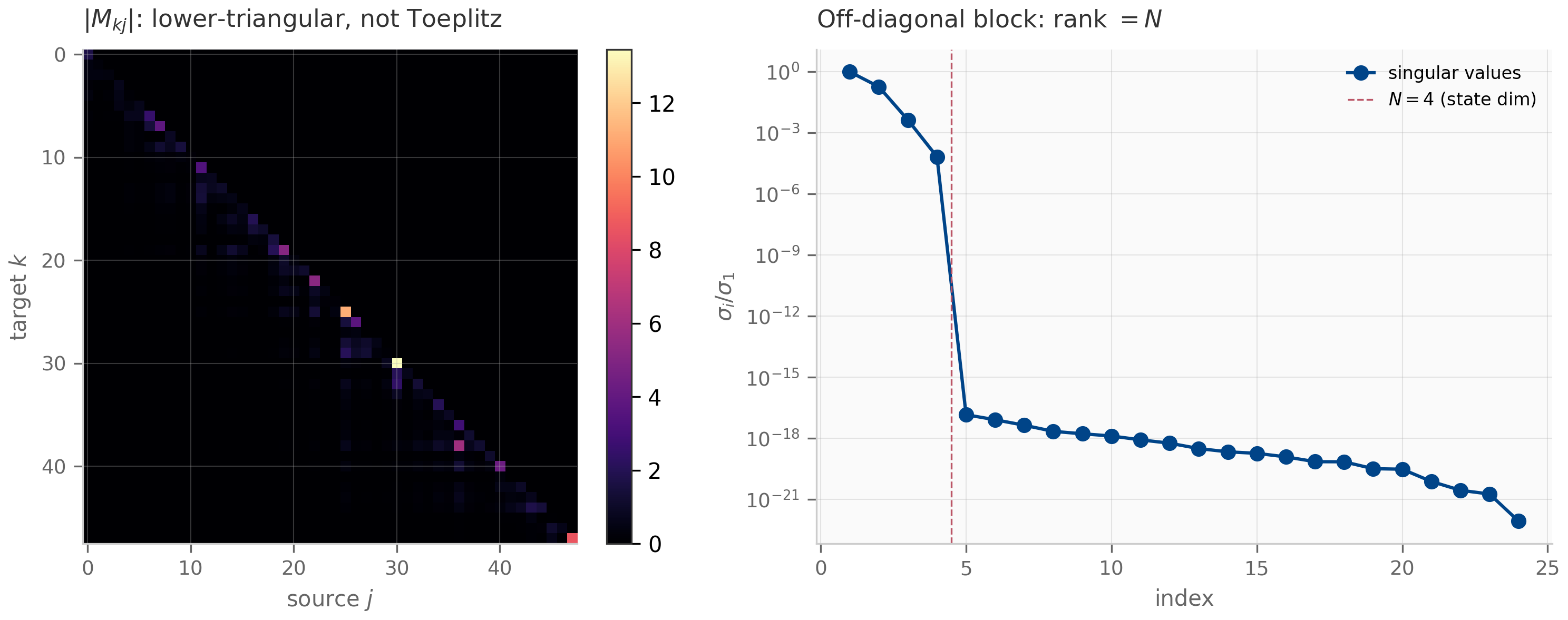
(LTI collapse.) If the discrete transition is input-dependent — for some — then the map is causal and linear, hence lower-triangular, but not Toeplitz: there is no single kernel with . The convolutional view of §8.3 exists if and only if the system is time-invariant.
The proof (Exercise 9.4, §9.9) is short: a causal linear map is a convolution exactly when its matrix has constant diagonals, and input-dependence makes even the main diagonal vary. The duality of §8.3 was a property of time-invariance all along; selectivity spends it.
9.2 Selective SSMs as discretized linear time-varying systems
The dynamical-systems name for what just happened is familiar. Chapter 8’s LTI SSM is the discretization of an autonomous linear system , whose coefficients do not depend on . A selective SSM is the discretization of a linear time-varying (LTV), or non-autonomous, system . The whole apparatus of §8.3 — a single , its powers , one kernel — assumed autonomy. LTV systems replace the matrix power with a matrix product.
(Discrete state-transition operator.) For the LTV recurrence with , the state is
where is the state-transition operator carrying state from step to step . The inputoutput map therefore has entry — a path-ordered product of transitions, not the power of the LTI case.
This is why no kernel exists: the tap from source to target depends on the entire path of step sizes between them, , and not on the offset . For a diagonal the product is elementwise and the per-mode transition is a clean exponential of an accumulated step, — the companion’s segsum computes exactly this cumulative decay. Reading the dynamics through the transition operator is the right altitude: it is what survives into §9.5 as the entries of a structured matrix, and it is what makes the LTV system non-Toeplitz but still cheaply structured.
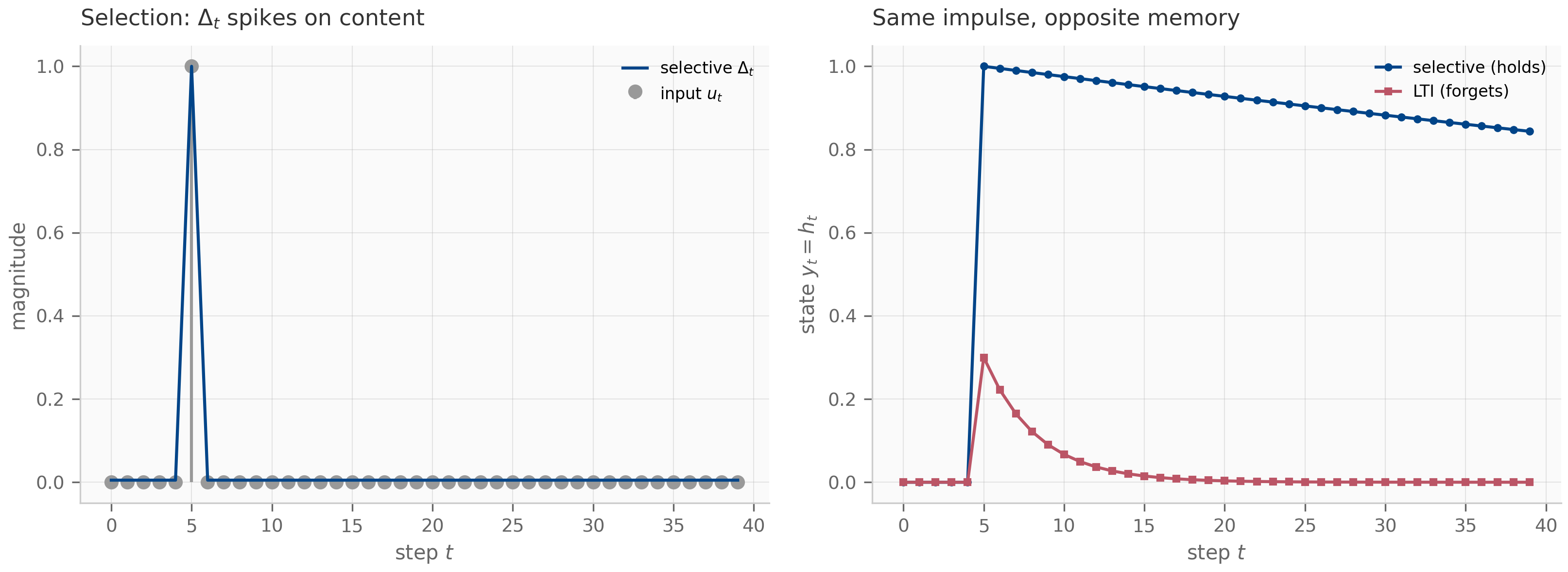
Selectivity is visible already in a single mode. Drive one stable mode with a content impulse and contrast a fixed- LTI system against a selective one whose gate opens ( large, : overwrite) on the content token and closes (, : hold) elsewhere. The selective system writes once and holds; the LTI system, forced to apply the same decay everywhere, forgets.
9.3 The selective scan: the §8.6 primitive, now the only route
The convolution is gone (Proposition, §9.1), so the FFT path of training-time S4 has no analogue here. What does survive is the parallel scan of §8.6 — and it survives because it never needed time-invariance in the first place. Recall the associative operator on pairs,
which composes “apply the first affine update, then the second.” Chapter 8 fed it the same at every step; nothing in the operator required that. Feeding it the time-varying pairs scans the selective recurrence directly. This is the selective scan.
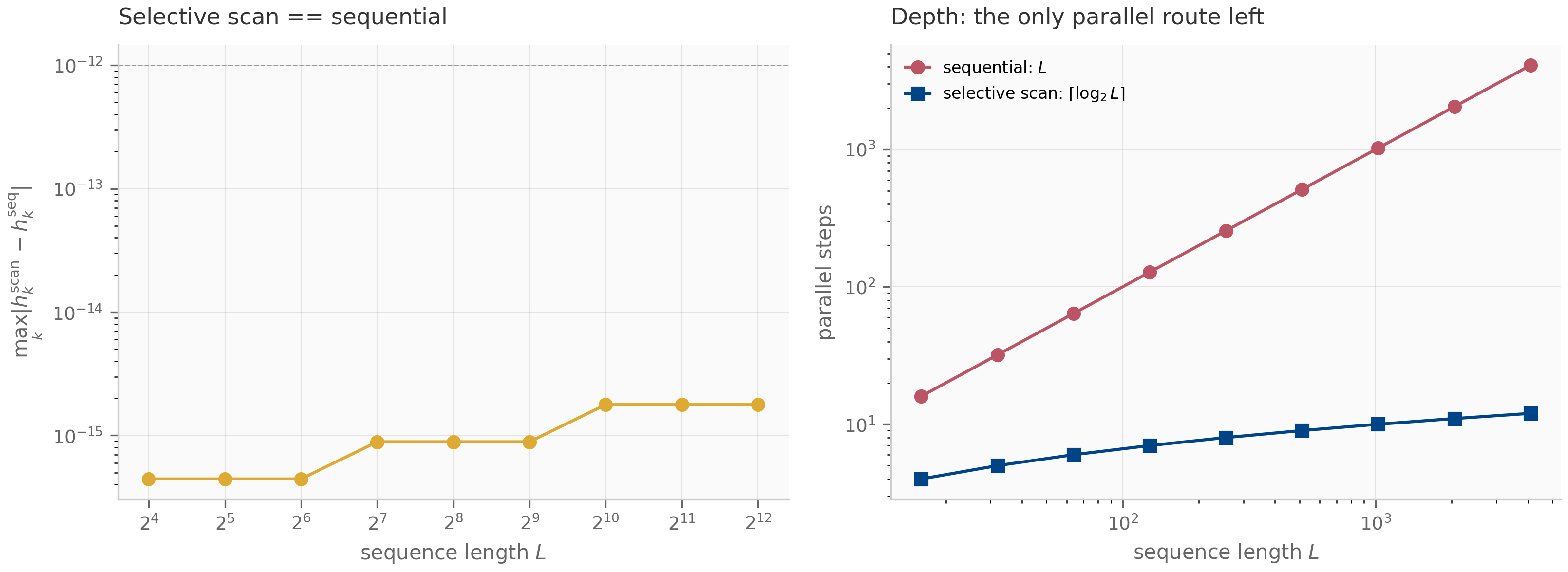
(Selective scan equivalence.) The operator is associative for arbitrary first components (not necessarily equal). Its inclusive prefix scan over has as its second components exactly the LTV states , computed in parallel depth Blelloch (1990) . Because no convolution exists (Proposition, §9.1), the FFT path of training-time S4 is gone; this scan recovers depth at linear work and is the primitive the layer is computed with. (Section 9.5 derives a second parallel route — a quadratic matrix multiply — from the same structure.)
The proof (Exercise 9.5, §9.9) is the §8.6 argument with one observation added: the associativity computation never used , so the LTI assumption was load-bearing only for the convolution, never for the scan. The companion pins the equivalence to machine precision — the selective associative scan and the sequential recurrence agree to a measured residual across sequence lengths, which test_selective_scan_equals_sequential holds below .
9.4 The hardware-aware fused kernel
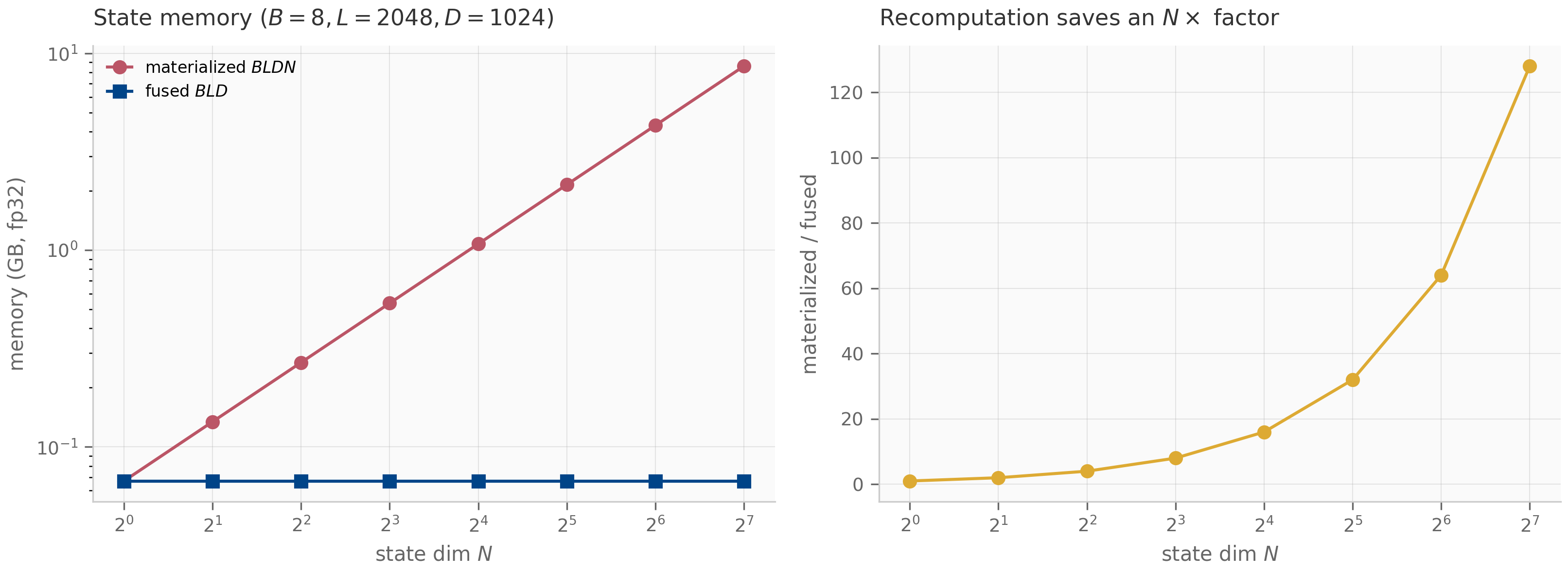
Making the scan the only route raises the stakes on computing it efficiently, and the obstacle is memory, not arithmetic. The selective scan’s state is per channel: for a batch of sequences of length with channels and state size , materializing every intermediate state — which the naive backward pass needs — costs , an blow-up over the inputs and outputs. At , , , that is 1.1 GB of fp32 state against 0.067 GB of output (figure below) — at Mamba’s working dimensions, the difference between fitting in memory and not.
Mamba’s selective-scan kernel resolves this with three hardware-aware moves Gu & Dao (2024)
. It fuses discretization, scan, and output projection into a single GPU kernel, so the expanded state is formed and consumed in fast on-chip SRAM and never written to slow HBM. It recomputes that state in the backward pass instead of storing it — the activation-recomputation trade that pays compute to save memory, the same jax.checkpoint discipline the Mamba-1 reference implementation applies to its selective-scan body. And it exploits the fact, from §9.3, that there is no convolution to fall back on: the scan must be fast, so the engineering goes into the scan rather than into an alternative path. The companion does not implement a CUDA kernel — it makes the memory accounting concrete (the figure above), which is the part that explains why the kernel exists.
9.5 Mamba-2 and SSD: the semiseparable-matrix view
Section 9.2 wrote the inputoutput map entry by entry. Collect those entries into a matrix and a second, matmul-friendly computation appears. Stacking with
and for , gives a lower-triangular matrix. This is the object Mamba-2 organizes the layer around, and it has exactly the structure that makes both computations cheap.
(Structured state-space duality.) For a diagonal state matrix , the selective-SSM output map is -semiseparable: every submatrix lying strictly below the diagonal has rank at most . Consequently admits two computations of the same result — a linear one, the recurrent scan of §9.3 in work and memory, and a quadratic one, forming and multiplying, in work using dense matrix multiplies.
The rank bound is the duality’s engine (Exercise 9.6, §9.9): writing the accumulated decay as with factors each strictly-lower block into a sum of rank-one outer products. The two computations trade off by regime: the recurrent (scan) mode wins for long sequences and autoregressive inference; the quadratic (matmul) mode wins for short chunks, because dense matrix multiplies are what tensor cores do fastest. Mamba-2’s production algorithm chunks the sequence and uses the quadratic mode within chunks and the linear mode across them — both unlocked by the same structure. The companion confirms the two modes agree to a measured residual (pinned below by test_recurrent_equals_matmul) and certifies the rank bound numerically.
9.6 Duality with linear attention
The semiseparable view pays its largest dividend when the state matrix is a scalar. Mamba-2 restricts — one shared decay per head — which makes the accumulated decay a scalar, , and factors the matrix entry into a decay times an inner product:
with the Hadamard product. Read the right-hand side as attention: are queries, are keys, is the score matrix, are values, and is a causal decay mask in place of softmax. Two things separate it from softmax attention. The mask is fixed by the accumulated step sizes between the two positions, not by a content–content interaction of and ; and the scores enter linearly — there is no softmax nonlinearity — which is precisely what lets the same operator also run in the linear-cost recurrent mode (§9.5). It is linear attention, not softmax attention.
(Selective SSM as masked linear attention.) For scalar , the selective SSM output equals , a masked linear attention with decay mask . The mask is 1-semiseparable (rank-one strictly-lower blocks). The recurrent scan and this masked matmul are the SSM and attention faces of one operator.
This is the formal sense in which “transformers are SSMs” Dao & Gu (2024)
: the linear-attention layer of Katharopoulos et al. Katharopoulos et al. (2020)
and the selective scan compute the same family of contractions, distinguished only by which mode — recurrent or quadratic — is run. The companion verifies the identity as a matrix equation, with the directly-built and the masked-attention form agreeing to (pinned below by test_scalar_A_equals_masked_attention), and certifies that is 1-semiseparable. Chapter 11 enters this same duality from the attention side — linear attention and the delta-rule lineage are the “transformer” reading of the structure this section reached from the SSM side.
9.7 What’s next
The thread of this chapter is one structural change and its consequences. Making depend on the input turns the LTI SSM into a linear time-varying system (§9.2); time-variance breaks the convolution–recurrence duality, so no single kernel exists (§9.1) and the §8.6 associative scan — fed input-dependent transitions — becomes the parallel primitive the layer is computed with (§9.3), which is why Mamba needs a fused, recompute-in-backward kernel (§9.4). Re-reading that scan as a matrix exposes its -semiseparable structure and the recurrent/quadratic duality (§9.5), and for scalar state that matrix is masked linear attention (§9.6).
Chapter 10 keeps selectivity and changes the discretization: Mamba-3 moves to a complex state and replaces zero-order hold with the exponential-trapezoidal scheme of Chapter 4 when the selective dynamics turn stiff Lahoti et al. (2026) . That chapter is where the symplectic-integrator pilot finds its empirical anchor — the selective layer built here, run with a second-order geometric integrator. Chapter 11 takes the §9.6 duality the other way, developing linear attention and the delta-rule lineage as the attention-side reading of the same structured contractions. The selective scan and the semiseparable matrix are the two objects everything downstream reuses.
9.8 Exercises
Six problems mixing computation and theory. Short/numerical (9.1–9.3) have inline collapsible solutions; the theory exercises (9.4–9.6) have full worked solutions in §9.9.
Exercise 9.1 (computation)
Take one stable mode with , and two step sizes: a “write” step and a “hold” step . (a) Compute the discrete transitions and . (b) A value written into the state then held for steps is multiplied by ; compute the retained fraction. (c) Contrast with an LTI system that must use for all steps. What does this say about selectivity?
Solution
(a) (gate nearly open: most of the old state is overwritten), (gate nearly closed: the state is held). (b) Holding for 20 steps retains , about . (c) The LTI system stuck at retains — total forgetting. Selectivity is precisely the freedom to make near on tokens worth holding and near on tokens worth overwriting; a fixed cannot do both, which is the §9.2 figure in two numbers.
Exercise 9.2 (code)
Run companions/ch09/jax/selective_scan_demo.py and confirm the selective associative scan matches the sequential recurrence (the companion reports a residual ). Then explain why the S4 trick of computing the same output by an FFT convolution is unavailable here, referencing Proposition (§9.1).
Solution
The associative scan and the sequential recurrence compute the identical linear recurrence by different reduction orders, so for the same they agree to floating-point error (the companion measures , pinned below ). The FFT path is unavailable because it computes a convolution , which requires a single kernel . By Proposition (§9.1) no such kernel exists once is input-dependent: the map is not Toeplitz, so it is not a convolution, so there is nothing to transform. The scan, by contrast, only needs the per-step pairs and an associative operator, neither of which assumes time-invariance (§9.3).
Exercise 9.3 (computation)
Consider a scalar-state () selective system of length with shared decay , step sizes , scalar projections . Write the entry of the SSD matrix for , and argue that any strictly-lower block (e.g. rows , columns ) has rank .
Solution
With , for . Write , so the accumulated decay is . Then for ,
The block on rows , columns is , an outer product of two vectors — rank . Every strictly-lower block factors the same way, so the matrix is -semiseparable.
Exercise 9.4 (theory) — solution in §9.9
Prove Proposition (§9.1): if the discrete transition is input-dependent, the causal linear map is not Toeplitz, so no convolution kernel with exists. (Hint: a causal linear map is a convolution iff its matrix has constant diagonals.)
Exercise 9.5 (theory) — solution in §9.9
Prove Proposition (§9.3): the operator is associative for arbitrary , and its inclusive prefix scan over reproduces the LTV states . Identify the single place the §8.6 argument used time-invariance and confirm the selective scan does not need it.
Exercise 9.6 (theory) — solution in §9.9
Prove Theorem (§9.5): for diagonal , every strictly-lower-triangular block of the SSD matrix has rank . Then specialize to scalar to derive the masked-attention form of Theorem (§9.6) and show is -semiseparable.
9.9 Full solutions to theory exercises
Solution to Exercise 9.4
A causal linear map on sequences of length is represented by a lower-triangular matrix with . It is a convolution — i.e. — if and only if depends only on the offset , which is exactly the statement that is Toeplitz (constant along each diagonal ).
For the selective system, the diagonal- entry is
Consider the main diagonal (offset ): the accumulated sum is empty, so . Because are input-dependent, varies with whenever the input does, so the main diagonal is not constant and is not Toeplitz. (More strongly, for the factor is not a function of once varies, so no off-diagonal is constant either.) A non-Toeplitz causal map is not a convolution, so no kernel exists; the time-invariant case, where makes depend only on , is the sole case that is Toeplitz.
Solution to Exercise 9.5
Associativity. Write a pair as the affine map (with acting elementwise). Composition of affine maps is associative because function composition is; concretely, with as defined,
and the two agree. Nowhere did this computation assume — that is the single place §8.6 silently used (and did not need) time-invariance. Prefix scan. Let and let be the inclusive scan. By induction on the second component of equals : for it is (from ); and has second component . Since is associative, all prefixes are computable by a balanced reduction tree in depth Blelloch (1990) . The selective scan is thus the §8.6 scan verbatim, with time-varying in place of a constant — the operator’s associativity never cared.
Solution to Exercise 9.6
Semiseparability. Fix a strictly-lower block: rows and columns with , so throughout and the accumulated sum is nonempty. Write , so and . Then
with and . As a matrix the block is with , , hence rank . Every strictly-lower block has this form, so is -semiseparable. (The factorization is exactly what the chunked algorithm exploits: is read out from the per-chunk states, folded into them.)
Scalar specialization. Put , i.e. for all . The decay no longer depends on , so it pulls out of the sum:
with . In matrix form , the masked-attention form of Theorem (§9.6): is the score matrix and the decay mask. Finally for , so any strictly-lower block of is the outer product — rank one. Thus is -semiseparable, and the full is -semiseparable with the state size (here the rank of the score matrix).
9.10 Companion code
Two language tracks for Chapter 9 — JAX (the reference, with the parallel selective scan and the semiseparable-matrix tools) and PyTorch (the nn.Module layers and the masked-attention dual). Julia is omitted, as in Chapter 8: the selective scan and the SSD matrix are the same algorithm in any language, and the JAX/PyTorch pair already carries the cross-framework lesson. The two tracks are pinned bit-for-bit against each other in float64.
JAX (companions/ch09/jax/):
selective_ssm.py— the SISO selective-SSM core: the selection mechanism, the per-step ZOH discretization, and the selective scan viajax.lax.associative_scanwith its sequential oracle. The §9.3 equivalence lives here.selective_vs_lti.py— emitsselective-vs-lti.png(§9.2): the held-vs-forgotten single-mode contrast.selective_scan_demo.py— emitsselective-scan.png(§9.3) andmemory-cost.png(§9.4): scan-vs-sequential agreement and depth, and the materialized-vs-fused memory accounting.ssd_semiseparable.py— the SSD tools:segsum, the semiseparable matrixbuild_ssm_matrix, the rank certificateis_n_semiseparable, and the scalar-masked_attention_form; emitssemiseparable.png(§9.5).tests/—test_selective.pypins the selective scan-equivalence, stability by construction, and the not-Toeplitz collapse;test_ssd.pypins the recurrent-vs-matmul duality, -semiseparability, and the scalar- masked-attention identity.
PyTorch (companions/ch09/torch/):
selective_ssm.py— the selective SSM as annn.Module(A_loga learnablenn.Parameter, selection projections asnn.Linear, eager sequential scan), plus the functional core mirrored from JAX.ssd_matmul.py— the scalar- dual form asSSDAttention: masked linear attention with the decay mask in place of softmax.tests/test_selective_torch.py— cross-framework parity: the torch selective scan and SSD matrices equal their JAX counterparts to within .
To run from the repo root:
# JAX (uses the uv .venv with jax, numpy, matplotlib)
PYTHONPATH=. python companions/ch09/jax/selective_vs_lti.py
PYTHONPATH=. python companions/ch09/jax/selective_scan_demo.py
PYTHONPATH=. python companions/ch09/jax/ssd_semiseparable.py

# PyTorch (needs the .venv [torch] extra)
PYTHONPATH=. python companions/ch09/torch/selective_ssm.py
PYTHONPATH=. python companions/ch09/torch/ssd_matmul.py
All figures emit to public/figures/ch09/.