Linear attention and Hyena: long convolution and gated recurrence
Linear attention read as a matrix-state linear recurrence — the dual of Chapter 9's scan, entered from the attention side — then gated into the LTV/selectivity face (GLA, RetNet), pivoted to Hyena's implicit LTI long convolution, and landed honestly on the associative-recall capacity limit of any finite state.
On this page
- 11.1 From softmax to separable scores
- 11.2 Linear attention as a matrix-state recurrence
- 11.3 Gating: GLA, RetNet, and the LTV reading
- 11.4 Hyena: the FFT long convolution
- 11.5 Implicit and selective filters
- 11.6 Counter-evidence: associative recall and capacity
- 11.7 What’s next
- 11.8 Exercises
- Exercise 11.1 (short)
- Exercise 11.2 (short, code)
- Exercise 11.3 (short)
- Exercise 11.4 (theory) — solution in §11.9
- Exercise 11.5 (theory) — solution in §11.9
- Exercise 11.6 (theory) — solution in §11.9
- 11.9 Full solutions to theory exercises
- Solution to Exercise 11.4
- Solution to Exercise 11.5
- Solution to Exercise 11.6
- 11.10 Companion code
Linear attention and Hyena: long convolution and gated recurrence
11.1 From softmax to separable scores
Chapter 9 reached a striking identity from the state-space side: a scalar-state selective SSM is masked linear attention (Theorem 9.5). The scan’s path-ordered taps reassemble into a single lower-triangular matrix , with a causal decay mask replacing the softmax. This chapter enters that same duality from the other side. We start with attention and rediscover the state space.
Causal attention computes, for each position ,
The exponential couples every query to every key: the normalizer cannot be factored across , so the only way to evaluate it is to materialize all scores. The move that breaks the coupling Katharopoulos et al. (2020) is to choose a feature map with non-negative entries and write the similarity as an inner product of features,
Separability is the whole engine. Because factors, the numerator and denominator each become a query contracted against a running sum over keys — and a running sum is a state.
11.2 Linear attention as a matrix-state recurrence
Fix . Define a matrix state and a normalizer by
with , . This is a bona fide state-space recurrence: the hidden state is a matrix, the transition is the identity (, pure accumulation with no forgetting — the LTI face of Chapter 8), and the input is injected as the rank-one outer product . It is Chapter 9’s scan with the carry promoted from a vector to a matrix and the decay switched off.
The same operator has a second, parallel face. Stacking and , the unnormalized output is a masked matrix product.
For any feature map , the recurrent form (, output ) and the parallel form
with the all-ones causal mask, compute the identical output. The recurrent form costs time and memory; the parallel form costs . This is exactly Theorem 9.5 with the decay mask specialized to ones.
The proof (Exercise 11.4, §11.9) is one line of reassociation: , so , which is precisely row of . The mask supplies the causal cumulative sum that the recurrence performs incrementally. The companion confirms the two routes agree to machine precision in float64: at , flat across sequence lengths.
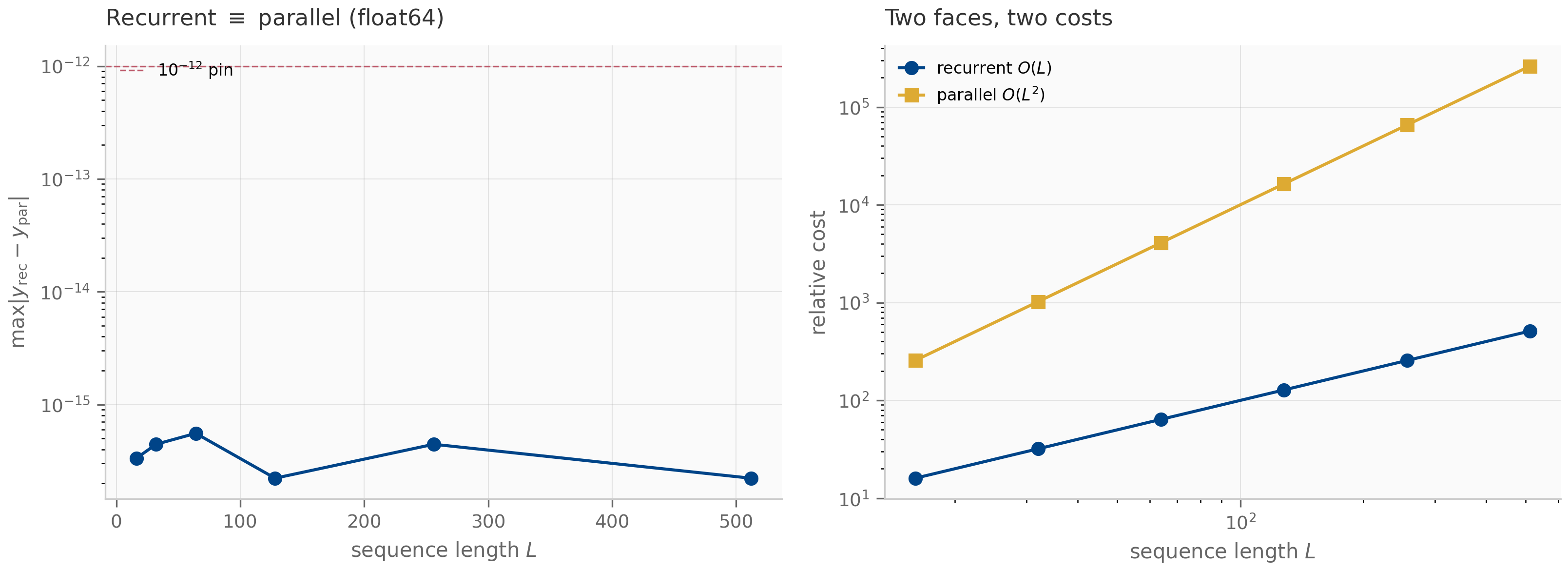
The normalizer, and why this chapter is float64. The denominator is a large-over-large quotient: both and the numerator grow like , so the ratio is a difference of accumulations prone to catastrophic cancellation in low precision. The recurrent and parallel forms accumulate that quotient in different orders (sequential cumsum versus a single matmul), so their agreement is a direct probe of arithmetic precision. In float64 they match to at ; in float32 the same computation caps out at — a precision gap of nearly . The identity pin is simply unreachable in single precision, which is why every companion in this chapter runs float64. (Gated linear attention in §11.3 sidesteps the issue by dropping the normalizer for an explicit decay plus an output normalization — cleaner numerically.)
11.3 Gating: GLA, RetNet, and the LTV reading
Ungated linear attention never forgets. To make it selective — to let the state forget — attach a per-step gate to the transition:
This is the Chapter 9 selectivity move read from the attention side. Two regimes sit inside it:
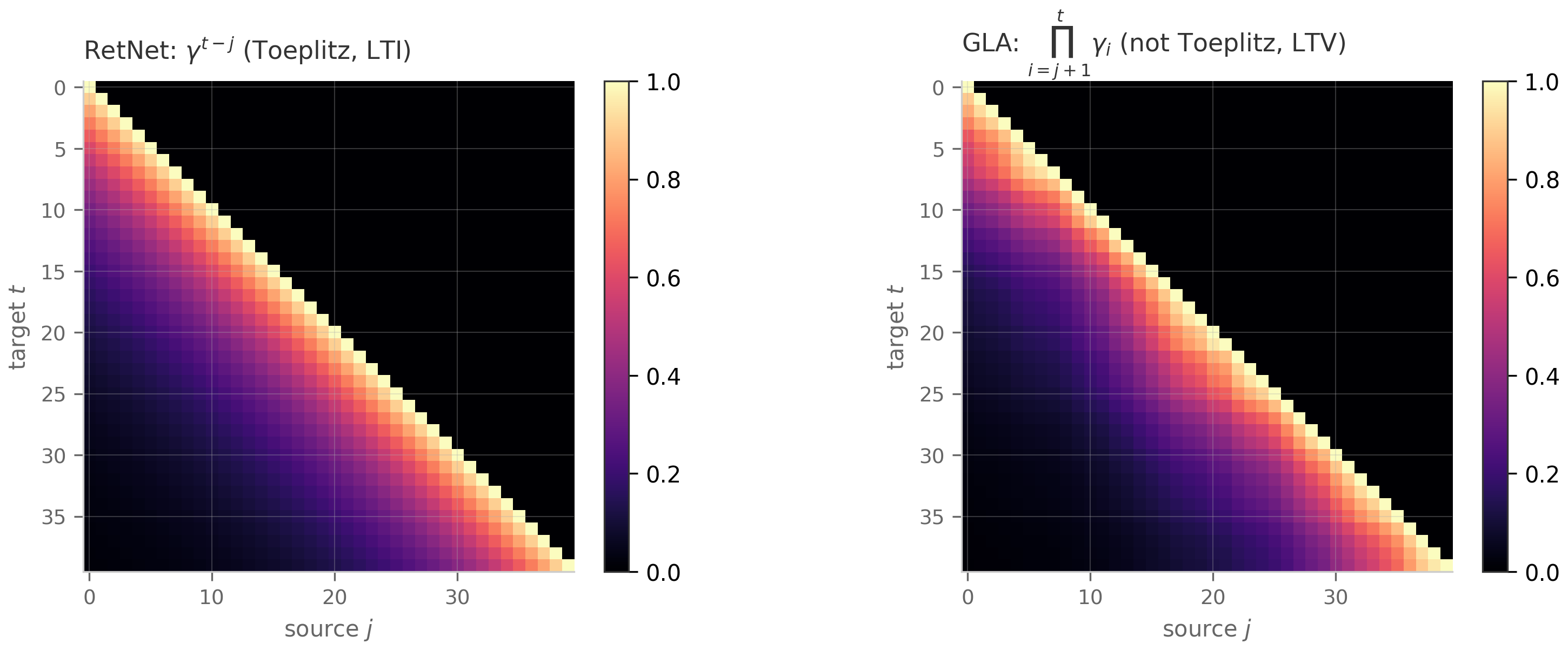
- RetNet Sun et al. (2023) takes , a fixed head-wise decay. The transition is constant, so the operator is LTI with forgetting — the Chapter 8 face plus a decay. Its parallel decay mask is Toeplitz (it depends only on the lag ).
- GLA Yang et al. (2024) and HGRN2 Qin et al. (2024) make data-dependent. The transition now changes every step, so the operator is LTV — input-dependent forgetting, exactly the selectivity of Chapter 9. Its decay mask is not Toeplitz; the diagonals vary, just as Chapter 9’s selective decay mask does.
The masked-parallel form generalizes by the GLA “secondary” rescaling: with the cumulative log-gate , set and ; then is the gated score. This is what makes the duality exact.
The gated recurrence , , has a masked-parallel form. For a scalar per-step gate it is exactly with the 1-semiseparable decay mask , and under this coincides exactly with the decay mask of Theorem 9.5 — gated linear attention and the scalar-state selective SSM are the same operator, read from opposite sides. For a per-feature gate the decay acts per channel and does not collapse to a single scalar mask; the parallel form instead rescales features by the cumulative gate (, , ), recovering the same recurrence (§11.9).
The proof is Exercise 11.5 (§11.9): unroll the gated recurrence, contract with
, and recognize the product-of-gates as the cumulative decay that
Theorem 9.4‘s segsum exponentiates. The companion both
checks the recurrent–masked identity ( difference for
a data-dependent gate) and verifies the cross-chapter bridge against the actual
Chapter 9 code: the GLA scalar mask and Chapter 9’s segsum mask agree to
(bit-identical) under .
11.4 Hyena: the FFT long convolution
The second operator family of this chapter abandons attention entirely — yet it is the same structural idea in new dress, not a digression: Hyena’s convolution is one more instance of the LTI/LTV fork that organized §§11.2–11.3, as §11.5 will make explicit. Hyena Poli et al. (2023) interleaves implicit long convolutions with elementwise multiplicative gating. The convolution is the object to teach: a causal long convolution is a linear time-invariant operator — the convolutional view of an SSM (Proposition 8.1) — computable in by the FFT rather than the explicit Toeplitz product. For input and a per-channel filter ,
The one subtlety is causality under the cyclic FFT.
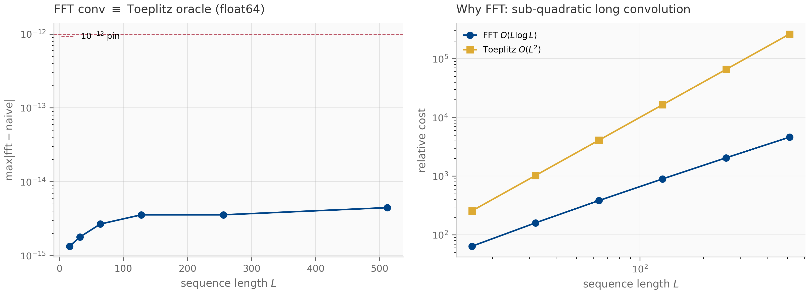
Padding and the filter to length , multiplying their real FFTs pointwise, inverse-transforming, and truncating to the first samples yields exactly the lower-triangular Toeplitz product above. Padding to (in fact any ) is sufficient: it sends the cyclic FFT’s wrap-around terms onto the zero-padded tail of , where they contribute nothing. The un-padded length- transform wraps late taps onto early outputs and breaks causality, so some padding past is required.
The proof is Exercise 11.6(a) (§11.9). The companion makes both halves concrete: the FFT route reproduces the explicit-Toeplitz oracle to in float64 (the predecessor implementation ran float32 at a tolerance — this is a tightening), while the un-padded variant disagrees with the oracle by , an violation of causality.
11.5 Implicit and selective filters
What does the long convolution mean in the dynamical-systems vocabulary of this book? Everything hinges on whether the filter is fixed or input-dependent.
When the filter is static across the batch and sequence, is a single linear time-invariant convolution — one kernel, the convolutional face of an SSM (Proposition 8.1). S4 lives exactly here: its kernel is materialized from a structured continuous-time ODE, and the same FFT machinery of §11.4 applies. Hyena keeps the unrestricted kernel and pays the factor, where S4 and Mamba fix the kernel shape — a structured semiseparable matrix (Theorem 9.4) — to buy .
When the filter is made input-dependent — the “selective Hyena” variant, where the convolution kernel itself is a function of the input — time-invariance breaks, exactly as Chapter 9’s input-dependent broke it. No single kernel exists; no convolution theorem applies; the operator rejoins the LTV family of §11.3. This is the same fork seen three times now: a fixed transition is LTI and admits a convolution or a closed-form mask; an input-dependent transition is LTV and admits only the scan. Hyena’s gating, GLA’s decay, and Mamba’s selection are three spellings of one move.
11.6 Counter-evidence: associative recall and capacity
Beyond-SSM does not mean better-than-SSM. The honest place to end is where linear attention loses: multi-query associative recall (MQAR) — store key–value pairs, then answer queries by retrieving the value bound to a key Arora et al. (2024) . On this task, linear attention degrades as grows while selective SSMs (Mamba) and softmax attention stay near-perfect. The mechanism is the §11.2 insight turned into a limitation, and it is provable.
The linear-attention state is a sum of rank-one matrices, so . If , the feature vectors are linearly dependent, so the readout cannot reproduce linearly independent values: there exist queries for which exact recall is impossible, regardless of . Capacity is bounded by the feature dimension.
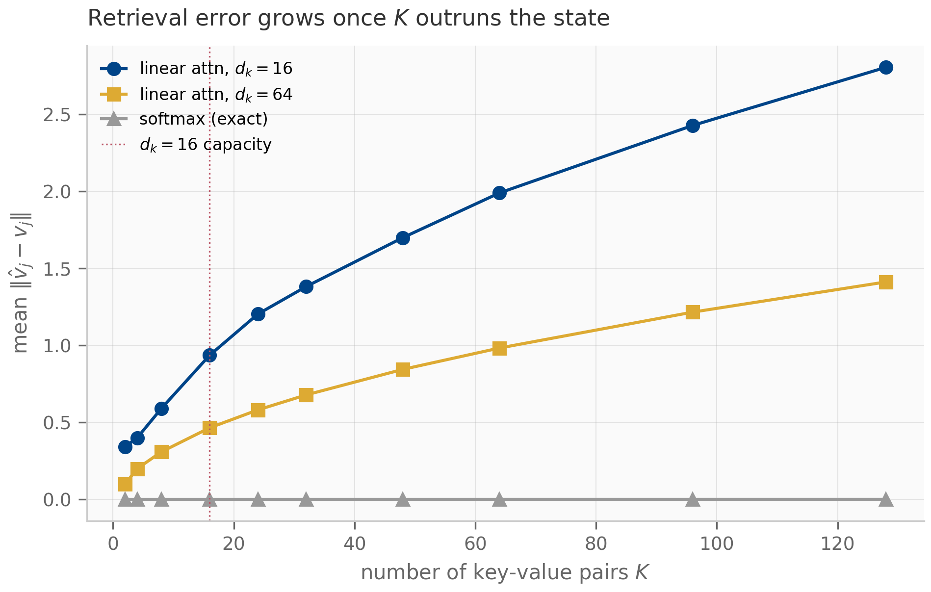
The proof is Exercise 11.6(b) (§11.9). The companion turns the bound into a measured fact (a fixed-weight mechanism, not a trained model — the trained-model accuracy curves are cited to Zoology Arora et al. (2024) ). Storing random unit keys with orthonormal values and reading each back, the per-binding retrieval error behaves exactly as the rank bound predicts:
- Below capacity, exact. With orthonormal keys the features are independent, the state is full-rank, and recall is exact — error .
- Past capacity, degrading. With generic keys the error grows like : at it is for and for (capacity scales with the state size), rising to at .
- The oracle stays exact. Softmax attention’s exponential sharpening concentrates the readout on the self-match, so its error is independent of — the capacity-unbounded baseline that linear attention cannot match.
Gating (§11.3) helps at the margin — a decay lets the state shed stale bindings — but it reweights a finite state, it does not raise the rank ceiling. Closing the gap needs either a genuinely larger structured state (the selective-SSM route of Chapters 9–10) or a smarter write rule, which is the subject of Chapter 12.
11.7 What’s next
This chapter built the linear-attention half of the “beyond-SSM” family: an additive matrix-state recurrence (), gated into the LTV/selectivity face (GLA, RetNet), with Hyena’s implicit LTI long convolution as the sibling operator and a hard capacity limit (§11.6) at the bottom.
Chapter 9 promised this chapter would develop “linear attention and the delta-rule lineage” as the attention-side reading of structured contractions. We have built the linear-attention half; the delta-rule half sharpens exactly the §11.6 capacity limit. Instead of blindly accumulating , the delta rule overwrites the value currently associated with a key — a rank-one correction
turning the identity-transition recurrence into a genuinely data-dependent write. That is Chapter 12 (the online-learning reading: DeltaNet as explicit-Euler, Longhorn as backward-Euler). Chapter 13 adds exponential gates and matrix memory (xLSTM, RWKV-7); Chapter 14 mixes these layers with attention into the production hybrids. The structure is one family; we are still mapping its faces.
11.8 Exercises
Three short problems (solutions inline) and three longer ones (solutions in §11.9).
Exercise 11.1 (short)
Take , , and two key–value pairs with scalar values. Write explicitly as a sum of two outer products, and verify by hand that the unnormalized readout for a query equals row of the masked-attention form .
Solution
(a matrix since is scalar). Then . Row of the masked form is with for — identical (taking ). The outer-product sum and the masked row are two evaluations of the same contraction.
Exercise 11.2 (short, code)
Run companions/ch11/jax/linear_attention.py. Confirm the
recurrent and parallel forms agree to , and explain in one sentence
why the mask here is all ones below the diagonal, whereas Chapter 9’s mask
carried a decay.
Solution
The script prints . The mask is all-ones because ungated linear attention has transition : nothing decays between positions, so the weight on key at query is for every . Chapter 9’s mask carried because its transition decays the contribution of older positions. Gating (§11.3) restores that decay.
Exercise 11.3 (short)
Show that a constant gate reduces the GLA decay mask to RetNet’s , and explain in one line why a constant gate makes the mask Toeplitz while an input-dependent does not.
Solution
. This depends only on the lag , so is constant along each diagonal — Toeplitz. With input-dependent the product depends on which steps are spanned, not just how many, so equal-lag entries on a diagonal differ — the mask is no longer Toeplitz. (The companion’s RetNet mask has Toeplitz residual exactly .)
Exercise 11.4 (theory) — solution in §11.9
Prove the recurrent–parallel equivalence of §11.2: the recurrent matrix-state form and the masked-parallel form compute the same output, and state the time/memory cost of each.
Exercise 11.5 (theory) — solution in §11.9
Prove the gated-linear-attention duality of §11.3, and identify the exact correspondence under which the scalar-gate GLA mask coincides with the Chapter 9 decay mask of Theorem 9.5.
Exercise 11.6 (theory) — solution in §11.9
(a) Prove the FFT-causality theorem of §11.4 — that padding past (to ) lets the FFT compute the causal convolution, while the un-padded transform does not. (b) Prove the rank bound of the §11.6 capacity proposition, and connect it to the growth of retrieval error in the §11.6 capacity figure.
11.9 Full solutions to theory exercises
Solution to Exercise 11.4
Unrolling the recurrence from gives . Hence
Row of the parallel form is , since . The two are identical. The recurrent form stores only and does work per step: time, memory. The parallel form materializes the score matrix: time.
Solution to Exercise 11.5
Unrolling the gated recurrence,
Contracting with , . Writing gives , so with and we get with . For a scalar gate , the mask is ; under this is , exactly the Theorem 9.5 mask . The off-diagonal blocks of have rank one (a product of a column and a row ), so is 1-semiseparable. The companion confirms the masks are bit-identical ( difference).
Solution to Exercise 11.6
(a) Zero-pad to length . The pointwise product of their DFTs is the cyclic convolution . For and (both zero beyond ), the index ranges over . A negative index wraps to , where the padded is zero — so wrapped terms contribute nothing, leaving , the causal linear convolution. With (no padding) the same wrap sends to , where is nonzero, injecting acausal terms. Hence any suffices (the companion uses ), while fails. The companion’s un-padded variant differs from the oracle by .
(b) is a sum of rank-one matrices, so ; it is also (its columns lie in ) and . Thus . If , the vectors are linearly dependent: some , so the readout is a fixed linear combination of the readouts for the other keys and cannot independently equal for arbitrary value assignments. Exact recall of independent bindings is therefore impossible. The growth in the §11.6 capacity figure is the quantitative shadow of this: with random unit keys the interference has terms each of size , so its norm scales as — zero only when the keys are orthonormal, which requires .
11.10 Companion code
The companions live in companions/ch11/{jax,torch,julia} and are float64
throughout (§11.2 explains why). The JAX modules are canonical and produce every
figure; the torch modules mirror them and are checked for cross-framework parity
to ; the Julia module ports Hyena’s convolution to a third language
using only the standard library.
# JAX (canonical; emits the four figures to public/figures/ch11/)
PYTHONPATH=. python companions/ch11/jax/linear_attention.py
PYTHONPATH=. python companions/ch11/jax/gated_linear_attention.py
PYTHONPATH=. python companions/ch11/jax/fftconv.py
PYTHONPATH=. python companions/ch11/jax/mqar_recall.py

# Tests: JAX identities (< 1e-12), torch parity (< 1e-9), Julia FFT identity
.venv/bin/pytest companions/ch11/jax companions/ch11/torch -q
julia --project=companions/ch11/julia companions/ch11/julia/runtests.jllinear_attention.py— the matrix-state recurrence and its masked-parallel twin (§11.2), the capacity-rank object (§11.6), and the float64-vs-float32 normalizer demonstration.gated_linear_attention.py— GLA/RetNet gating, the decay masks, and the cross-chapter bridge to Theorem 9.5 built on Chapter 9’s ownsegsum(§11.3).fftconv.py— Hyena’s -padded FFT convolution against the explicit Toeplitz oracle, plus the un-padded variant that fails causality (§11.4). The torch port documents the buffers-vs-Parameters distinction (a fixed mask is a buffer; a learned filter is a Parameter).mqar_recall.py— the fixed-weight associative-recall mechanism behind §11.6: exact recall below capacity, degradation above it, and the softmax oracle at zero error.