Stability theory: Lyapunov, A-stability, BIBO

2.1 Three notions of stability

For the rest of this chapter, the system under analysis is the LTI state-space model from Chapter 1:

with $\statemat \in \R^{N \times N}$. The three notions:

1. Lyapunov stability asks: with $u \equiv 0$, do trajectories $\statevec(t) = e^{\statemat t} \statevec_0$ stay bounded as $t \to \infty$? Asymptotically stable if $\statevec(t) \to 0$.
2. A-stability is a property of a numerical integrator, not of the system. It asks: does the integrator preserve Lyapunov stability for every stable LTI test problem, at every step size $\stepsize > 0$? If yes, the method is A-stable.
3. BIBO stability asks: for the input–output mapping $u \mapsto y$, does every bounded input ($\sup_t \abs{u(t)} < \infty$) produce a bounded output? The system is BIBO-stable if yes.

When $\statemat$ has all eigenvalues in the open left half-plane (LHP), all three coincide for the LTI case. But:

• Lyapunov-stable systems can be Lyapunov-stable but not asymptotically stable (centers: pure imaginary eigenvalues, oscillations don’t decay).
• A-stability is a integrator property; the explicit Euler method is not A-stable, while the implicit Euler method is. The same continuous system therefore may need a stable integrator to preserve its stability.
• BIBO depends on the transfer function $H(s) = \outputmat (sI - \statemat)^{-1} \inputmat$ and on the choice of $(\statemat, \inputmat, \outputmat)$ realization. Two systems with the same $\statemat$ can have different BIBO properties if their $\outputmat$ “hides” unstable modes.

The rest of the chapter develops each notion in turn.

2.2 Lyapunov stability: theory

We restrict to the homogeneous case $\ddt \statevec = \statemat \statevec$ (zero input). The eigenvalue criterion is essentially the content of Chapter 1, §1.2, formalized:

The proof reduces to the matrix-exponential formula. If $\statemat = V \Lambda V^{-1}$ is diagonalizable, then $\statevec(t) = V e^{\Lambda t} V^{-1} \statevec_0$ and the $i$-th eigencomponent decays like $e^{\Re(\lambda_i) t}$. The Jordan-block caveat in case (1) handles the case where a defective imaginary eigenvalue produces polynomial growth in $t$ even though the real part is zero.

For nonlinear systems, the local-linearization picture from Chapter 1, §1.4 makes the same theorem applicable at each fixed point: the fixed point is asymptotically stable if the Jacobian’s eigenvalues all sit in the LHP. This is the principle that makes “check the eigenvalues” the first move in nearly every SSM stability analysis.

The Lyapunov equation

There’s an alternative characterization of asymptotic stability that doesn’t require computing eigenvalues. The continuous-time Lyapunov equation

(with $Q$ a given symmetric positive-definite matrix) has a unique symmetric positive-definite solution $P$ if and only if $\statemat$ is asymptotically stable. The function $V(\statevec) = \statevec^\top P \statevec$ is then a Lyapunov function for the system: $\dot V = -\statevec^\top Q \statevec < 0$ for all nonzero $\statevec$, so $V$ decreases along trajectories and forces them to the origin.

For SSM analysis, the Lyapunov-equation view is occasionally useful — for example, the controllability and observability Gramians of an LTI realization are Lyapunov solutions Antoulas (2005) — but the eigenvalue criterion is the more direct tool.

2.3 Lyapunov exponents: computation

The eigenvalues of $\statemat$ work as a stability diagnostic for LTI systems, where $\statemat$ is constant. For systems where the linearization $\jacobian(t)$ varies with time (e.g. a trained recurrent network in inference mode, where the per-step Jacobian depends on the input), eigenvalues at any single $t$ don’t tell the long-run story. The right tool is the Lyapunov exponent, which generalizes the eigenvalue’s real part to time-varying systems.

Three things make Lyapunov exponents the right object:

1. They generalize eigenvalues to time-varying systems. For a constant Jacobian $\jacobian_t \equiv \statemat$, $\lyapexp_i = \log\abs{\mu_i(\statemat)}$ where $\mu_i$ are the eigenvalues’ magnitudes (in the discrete case) or $\Re(\lambda_i)$ (in the continuous case). The connection back to Chapter 1’s eigenvalue classification is exact in the autonomous case.
2. The maximal Lyapunov exponent $\lyapexp_1$ measures sensitive dependence. A positive $\lyapexp_1$ means infinitesimally close initial conditions diverge exponentially (chaos); $\lyapexp_1 = 0$ is the edge-of-chaos regime; $\lyapexp_1 < 0$ means contracting dynamics.
3. They are robust to coordinate changes. Eigenvalues of the per-step Jacobian depend on the basis you write the state in; Lyapunov exponents do not.

The QR algorithm

Computing $\sigma_i(\Phi_T)$ for large $T$ directly is numerically impossible: even for a well-behaved system with $\lyapexp_1 = 0.1$, after $T = 100$ steps the largest singular value is $e^{10} \approx 22000$ and the smallest may be $e^{-10} \approx 5 \times 10^{-5}$. The product matrix $\Phi_T$ becomes either numerical zero or numerical infinity in finite-precision arithmetic, and finite-precision singular values lose all meaning. The fix, due to Benettin et al. Benettin et al. (1980) , is to factor the growth out at every step using QR decomposition.

The QR-based Lyapunov algorithm (the version that has become standard in dynamical-systems software):

Initialize Q_0 = I (identity), running sums L_i = 0 for i = 1..N.
For t = 1, 2, ..., T:
    M_t = J_t @ Q_{t-1}             # one-step forward propagation
    Q_t, R_t = qr(M_t)              # extract orthogonal + upper triangular
    Update L_i += log |R_t[i,i]| for each i
At the end:
    Lyapunov_i = L_i / T

The key insight: by re-orthonormalizing the propagated frame at every step, we factor the exponential growth into the diagonal of the upper-triangular $R_t$ rather than letting it accumulate in $\Phi_T$. The diagonal entries of $R_t$ are well-conditioned numbers near 1, and their logarithms sum nicely to give the Lyapunov exponents.

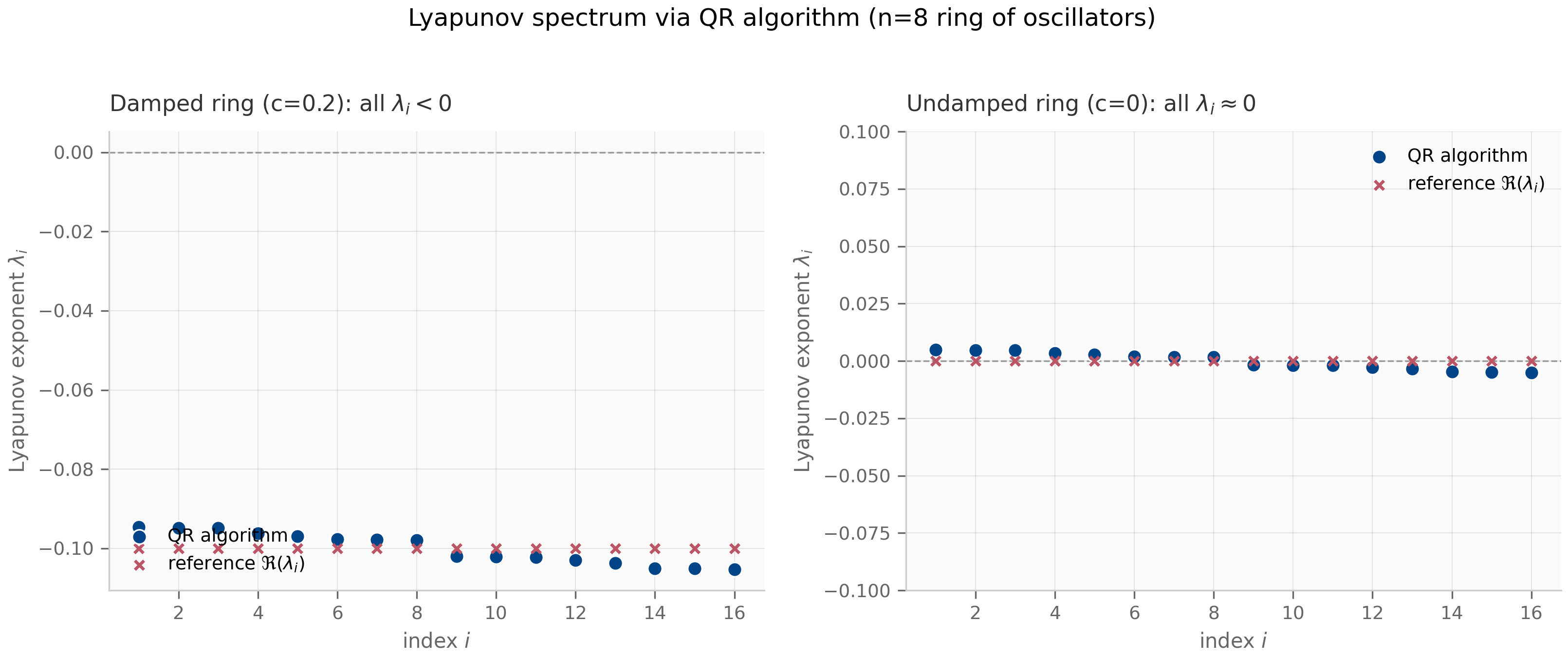
The companion lyapunov_qr.py implements this algorithm and applies it to the ring of coupled oscillators from Chapter 1, §1.4. The resulting spectrum’s structure — all exponents negative for the damped case, all near zero for the undamped case — matches the eigenvalue analysis exactly, validating the implementation.

2.4 A-stability: integrator regions of absolute stability

Switch perspectives. We now have a continuous system $\ddt \statevec = \statemat \statevec$ and we discretize it with some numerical integrator at step size $\stepsize$. The integrator approximates the true continuous trajectory by a discrete recurrence

where $R(z)$ is the integrator’s stability function, evaluated at the matrix argument $\stepsize \statemat$ via the matrix-functional-calculus convention. Different integrators give different $R$:

• Forward (explicit) Euler: $\statevec_{n+1} = \statevec_n + \stepsize \statemat \statevec_n$, so $R_{\text{FE}}(z) = 1 + z$.
• Backward (implicit) Euler: $\statevec_{n+1} = \statevec_n + \stepsize \statemat \statevec_{n+1}$, giving $R_{\text{BE}}(z) = 1/(1-z)$.
• Bilinear (Tustin / trapezoidal): $R_{\text{bil}}(z) = (1 + z/2)/(1 - z/2)$.
• Exact (zero-order hold): $R_{\text{ZOH}}(z) = e^z$. This is the integrator S4 uses by default.

The discrete recurrence is Lyapunov-stable if and only if every eigenvalue $\mu_i$ of $R(\stepsize \statemat)$ satisfies $\abs{\mu_i} \le 1$ (the discrete-time analog of the LHP criterion is the unit disk). Since the eigenvalues of $R(\stepsize \statemat)$ are $R(\stepsize \lambda_i)$ where $\lambda_i$ are the eigenvalues of $\statemat$, the question reduces to: for which $z = \stepsize \lambda_i$ in the complex plane is $\abs{R(z)} \le 1$?

A-stability matters because it means: if the continuous system is asymptotically stable, the integrator preserves that stability at every step size $\stepsize > 0$. Without A-stability, you have to pick $\stepsize$ small enough that $\stepsize \lambda_i$ lands inside the (bounded) stability region.

The four examples above:

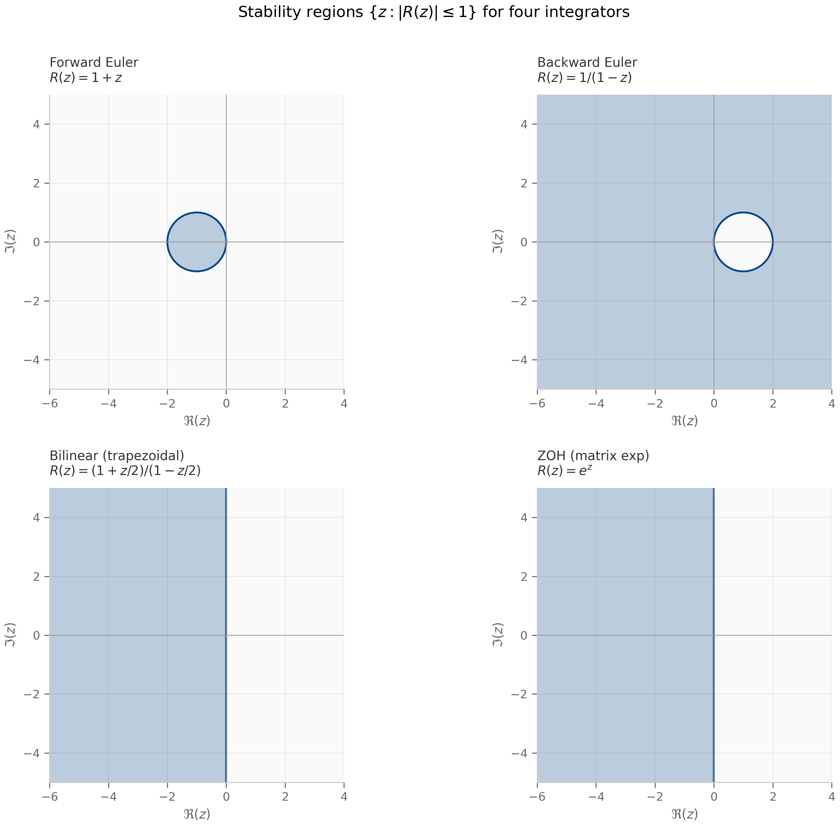
• Forward Euler: $\abs{1 + z} \le 1$ ⇔ $z$ in the closed disk of radius 1 around $-1$. Tiny region; not A-stable. For a continuous system with eigenvalue $\lambda = -100$ (fast decay), forward Euler requires $\stepsize < 2/100$ to avoid blowup.
• Backward Euler: $\abs{1/(1-z)} \le 1$ ⇔ $\abs{1-z} \ge 1$ ⇔ $z$ outside the open disk of radius 1 around $1$. This contains the entire closed LHP. A-stable.
• Bilinear (trapezoidal): $\abs{R_{\text{bil}}(z)} \le 1$ ⇔ $\Re(z) \le 0$ exactly. The stability region is exactly the closed LHP. A-stable, and the boundary coincides with the imaginary axis — a property called L-stability when combined with $R(z) \to 0$ as $\Re(z) \to -\infty$, which bilinear does not satisfy ($R_{\text{bil}}(-\infty) = -1$).
• Zero-order hold (matrix exponential): $\abs{e^z} = e^{\Re(z)} \le 1$ ⇔ $\Re(z) \le 0$. The stability region is the closed LHP. A-stable and L-stable. This is the gold standard for LTI discretization — and it’s what S4 uses internally.

Why this matters for SSMs

The S4 family uses ZOH discretization, and is therefore stable at every step size for which the continuous system is stable. Mamba-1 uses ZOH as well. Mamba-3’s exponential-trapezoidal rule (Chapter 10) is a second-order generalization of bilinear that retains A-stability. The C1 research pilot (see Chapter 6) asks whether symplectic integrators — A-stable methods designed to preserve geometric invariants — can do better for complex-state SSMs whose $\statemat$ has near-imaginary eigenvalues.

When a stability-region analysis fails, it usually fails dramatically: a forward-Euler discretization of a stiff system blows up in a handful of steps. This is exactly the failure mode that careful integrator choice prevents.

For full coverage of A-stability theory and a wider zoo of integrator stability functions, Hairer–Wanner’s stiff-systems volume Hairer & Wanner (1996) is the canonical reference.

2.5 BIBO stability

The third notion looks at the input–output mapping rather than the autonomous dynamics. For the system $\ddt \statevec = \statemat \statevec + \inputmat u$, $y = \outputmat \statevec$, the output under a unit-impulse input is the impulse response

The system is BIBO-stable if its impulse response satisfies $\int_0^\infty \norm{h(t)} \, dt < \infty$, equivalently if $h \in L^1$. Under this condition, any bounded input $u$ produces a bounded output $y$ — Young’s inequality on convolutions gives the precise bound $\sup_t \norm{y(t)} \le \norm{h}_{L^1} \cdot \sup_t \abs{u(t)}$.

Poles of $H(s)$ are the values of $s$ where $\det(sI - \statemat) = 0$ — i.e. the eigenvalues of $\statemat$ — unless a pole–zero cancellation occurs because $\outputmat$ doesn’t “see” some eigenmode. This cancellation matters: a system can be internally unstable (some $\lambda_i$ in the right half-plane) but BIBO-stable if those unstable modes are unobservable from $\outputmat$ and unreachable from $\inputmat$. The Kalman canonical-decomposition theorem makes this precise; for our purposes, the eigenvalues of $\statemat$ in the LHP are sufficient for both internal and BIBO stability.

For an SSM viewed as a sequence-to-sequence map, BIBO is the natural input–output stability concept: bounded inputs (typical of token embeddings) should produce bounded outputs (typical of pre-softmax logits). When training an SSM produces an $\statemat$ whose eigenvalues drift into the right half-plane, both internal (Lyapunov) and input–output (BIBO) stability fail simultaneously, and the model’s outputs blow up. Tracking the eigenvalues of $\statemat$ during training is therefore a single diagnostic for both failure modes.

2.6 Connection to Lyapunov functions

The Lyapunov-function method gives a non-spectral way to prove stability. For nonlinear systems where eigenvalues don’t directly apply, finding a function $V: \R^N \to \R$ with $V(0) = 0$, $V(\statevec) > 0$ for $\statevec \ne 0$, and $\dot V(\statevec) := \nabla V(\statevec) \cdot f(\statevec) < 0$ for all $\statevec \ne 0$ proves asymptotic stability of $\statevec^* = 0$.

For our LTI case $f(\statevec) = \statemat \statevec$, the Lyapunov equation $\statemat^\top P + P \statemat = -Q$ (with $Q$ p.d.) gives $V(\statevec) = \statevec^\top P \statevec$ as a quadratic Lyapunov function — and its existence with $P$ p.d. is equivalent to asymptotic stability (as noted in §2.2). The interest in the function-method picture for our context is mainly conceptual: it explains why “energy” arguments work to prove stability of mechanical systems (the energy is the Lyapunov function), and it generalizes immediately to nonlinear systems where the eigenvalue criterion only gives local information at fixed points.

This connects forward to Chapter 6, where the question of which discretization preserves a Lyapunov function (or, more strongly, an energy invariant) leads naturally into symplectic methods.

2.7 What’s next

Chapter 3 develops the structured-linear-algebra vocabulary (SVD, Jordan form, condition number, Toeplitz/Vandermonde/Cauchy/semiseparable structure) needed for the SSM kernel constructions in Chapters 7–9. Chapter 4 takes the discretization story started in §2.4 and develops it systematically: order conditions, accuracy classes, the Butcher tableau, the bilinear and ZOH derivations in detail. Chapter 6 picks up the A-stability theme and pushes into implicit and structure-preserving integrators — symplectic schemes, geometric integration, and the C1 pilot’s home territory.

2.8 Exercises

Six problems. Inline-collapsible solutions for the shorter ones; full solutions for the longer theory problems in §2.9.

Exercise 2.1 (computation)

Use the eigenvalue criterion (Theorem 2.1) to classify the stability of $\ddt \statevec = \statemat \statevec$ for $\statemat = \begin{pmatrix} -1 & 4 \\ -1 & -1 \end{pmatrix}$.

Exercise 2.2 (computation)

For the matrix $\statemat = \begin{pmatrix} 0 & 1 \\ -1 & 0 \end{pmatrix}$ of Exercise 1.1, find the eigenvalues and classify the Lyapunov stability. Is the system asymptotically stable?

Exercise 2.3 (computation)

The forward Euler method has stability function $R(z) = 1 + z$. For the continuous test problem $\dot x = \lambda x$ with $\lambda = -10$ (a stiff system with fast time scale), find the maximum step size $\stepsize$ for which forward Euler is stable.

Exercise 2.4 (computation)

Show that the bilinear method $R_{\text{bil}}(z) = (1 + z/2)/(1 - z/2)$ maps the closed left half-plane $\{\Re(z) \le 0\}$ onto the closed unit disk $\{\abs{w} \le 1\}$. (This is the Möbius map picture of the bilinear transform.)

Exercise 2.5 (theory) — solution in §2.9

State and prove the Lyapunov equation characterization of asymptotic stability: $\statemat$ is asymptotically stable iff for every symmetric positive-definite $Q$, the equation $\statemat^\top P + P \statemat = -Q$ has a unique symmetric positive-definite solution $P$.

Exercise 2.6 (theory) — solution in §2.9

Prove the BIBO criterion of Theorem 2.3: a causal LTI system is BIBO-stable iff all poles of its transfer function lie in the open left half-plane. (Hint: Use the Laplace-transform / convolution duality, and exploit the representation of the impulse response as a sum of exponentials.)

2.9 Full solutions to theory exercises

Solution to Exercise 2.5

Forward direction (Lyapunov equation ⇒ asymptotic stability): Suppose $P$ is symmetric positive-definite and satisfies $\statemat^\top P + P \statemat = -Q$ for some symmetric positive-definite $Q$. Define $V(\statevec) = \statevec^\top P \statevec$. Then $V > 0$ for $\statevec \ne 0$ (since $P \succ 0$), and along trajectories $\ddt \statevec = \statemat \statevec$:

So $V$ is a strict Lyapunov function and trajectories satisfy $V(\statevec(t)) \le V(\statevec(0)) e^{-\alpha t}$ for $\alpha > 0$ determined by the smallest eigenvalue of $Q$ over the largest of $P$. Hence $\statevec(t) \to 0$ and the origin is asymptotically stable.

Reverse direction (asymptotic stability ⇒ Lyapunov equation has p.d. solution): Suppose $\statemat$ is asymptotically stable. Define

The integral converges absolutely because $e^{\statemat t}$ decays exponentially. $P$ is symmetric (transpose preserves the integrand structure) and positive-definite (since $Q \succ 0$ and $e^{\statemat t}$ is invertible). Direct computation:

using the decay of $e^{\statemat t}$ at $\infty$. Uniqueness of $P$ follows from the linearity of the Lyapunov operator $\mathcal{L}(P) := \statemat^\top P + P \statemat$ and the fact that its kernel is trivial when $\statemat$ has no purely imaginary eigenvalues. ∎

Solution to Exercise 2.6

(⇒) BIBO-stable implies poles in open LHP. Suppose the system is BIBO-stable, i.e. $h \in L^1$. The Laplace transform $H(s) = \int_0^\infty h(t) e^{-st} dt$ then exists and is analytic for $\Re(s) \ge 0$ (since the integrand is bounded by $\abs{h(t)}$ which is integrable, the integral converges uniformly). $H$ is rational (the matrix-inverse formula gives $H(s) = \outputmat (sI - \statemat)^{-1} \inputmat$, a ratio of polynomials with denominator $\det(sI - \statemat)$). A rational function analytic on the closed right half-plane has no poles there — so all poles of $H(s)$ lie in the open LHP.

(⇐) Poles in open LHP implies BIBO-stable. Suppose all poles of $H(s)$ lie in the open LHP. Partial-fraction decomposition gives $H(s) = \sum_k \frac{c_k}{(s - p_k)^{m_k}}$ where $p_k$ are the poles with multiplicity $m_k$, and $\Re(p_k) < 0$ for all $k$. The inverse Laplace transform of each term is $\frac{c_k t^{m_k - 1}}{(m_k - 1)!} e^{p_k t}$, which is $L^1$ on $[0, \infty)$ because the exponential decay beats any polynomial growth in $t$. Sum of $L^1$ functions is $L^1$, so $h \in L^1$ and BIBO holds.

(For the multi-input multi-output case, apply the same argument entrywise to $H(s) \in \C^{M \times D}$.) ∎

2.10 Companion code

Two runnable companions in companions/ch02/jax/:

• lyapunov_qr.py — implements the QR-based Lyapunov-exponent algorithm and applies it to the ring-of-oscillators system from Chapter 1
• stability_regions.py — plots the regions of absolute stability for forward Euler, backward Euler, bilinear (trapezoidal), and ZOH in the complex plane

To run from the repo root:

PYTHONPATH=. python companions/ch02/jax/lyapunov_qr.py
PYTHONPATH=. python companions/ch02/jax/stability_regions.py

Figures land in public/figures/ch02/ (referenced from §2.3 and §2.4 above).