Niche-pilot integration: from curriculum to research output

17.1 What the dynamical-systems lens set out to earn

The book’s thesis has been a single sentence applied sixteen times: a sequence layer is a dynamical system, and you understand it by reading its state. A linear recurrence is a discretized ODE (Definition 1.1); its stability is the spectrum of its transition (Definition 2.2); its capacity is the rank of its state (Proposition 11.4); what it can losslessly recall is set by its state’s bit budget (Proposition 15.1). The claim was never that this lens is the only one — it is that it earns its keep as a research instrument, letting a numerical analyst ask questions about sequence models in their native vocabulary.

A thesis like that is proven by use, not assertion. The curriculum was designed around two research pilots that put the lens to work, and this chapter is where the book’s pieces compose into them:

• C1 — symplectic and geometric integrators for SSMs (the primary pilot): does a trained SSM’s transition have enough Hamiltonian structure that a structure-preserving integrator would beat the exp-trapezoidal default of Mamba-3? This is the question only the geometric-integration lens can ask (Chapters 1–3, 6, 10).
• B — synthetic two-timescale benchmarks (the parallel pilot): can an architecture cleanly disentangle a fast process from a slow one, and does its effective state size predict whether it can? This composes the singular-perturbation view Kokotović et al. (1986) (Chapter 14), the diagnostics (Chapter 15), and the protocol (Chapter 16).

Two boundaries govern everything that follows, and the chapter marks them everywhere. First, cited versus demonstrated: results we prove or measure are ours; the deep ceilings (the $\mathsf{TC}^0$ impossibility, Merrill et al. (2024) ) are cited. Second, and more load-bearing here, idealized versus trained: every demonstration in this chapter runs on a constructed system with a known answer — an oscillator mode, a known HMM. Turning these instruments on trained checkpoints is the pilots’ empirical program, in flight, not reported here. The chapter ships the reproducible template; the data is forthcoming.

17.2 C1 — symplectic integrators, and an atlas cell

Chapter 6 built the modified-Hamiltonian theory of symplectic integration Hairer et al. (2006) (Theorem 6.2): a symplectic step conserves a perturbed energy exactly, so its energy error stays in a bounded band forever, while a non-symplectic step of the same order lets energy drift secularly (Figure 6.2). Chapter 10 built Mamba-3’s complex-mode SSM Lahoti et al. (2026) and its exp-trapezoidal discretization (Theorem 10.1, Theorem 10.3). The C1 pilot’s opening question fuses them: if a trained SSM mode is near-conservative, is the exp-trapezoidal rule leaving structure on the table that a symplectic integrator would keep?

The bridge is exact. The harmonic oscillator $\dot q = p,\ \dot p = -q$, written as a complex state $z = q + ip$, obeys $\dot z = -iz$ — a Mamba-3 complex mode at the purely imaginary eigenvalue $\lambda = -i$. A near-conservative SSM mode is the same mathematics on a new object, not an analogy — which is what makes C1 a direct transfer of the geometric-integration toolkit rather than a metaphor for it.

The atlas cell measures three integrators of this one mode, composing Chapter 6’s Verlet and RK4 steppers with Chapter 10’s exact complex recurrence:

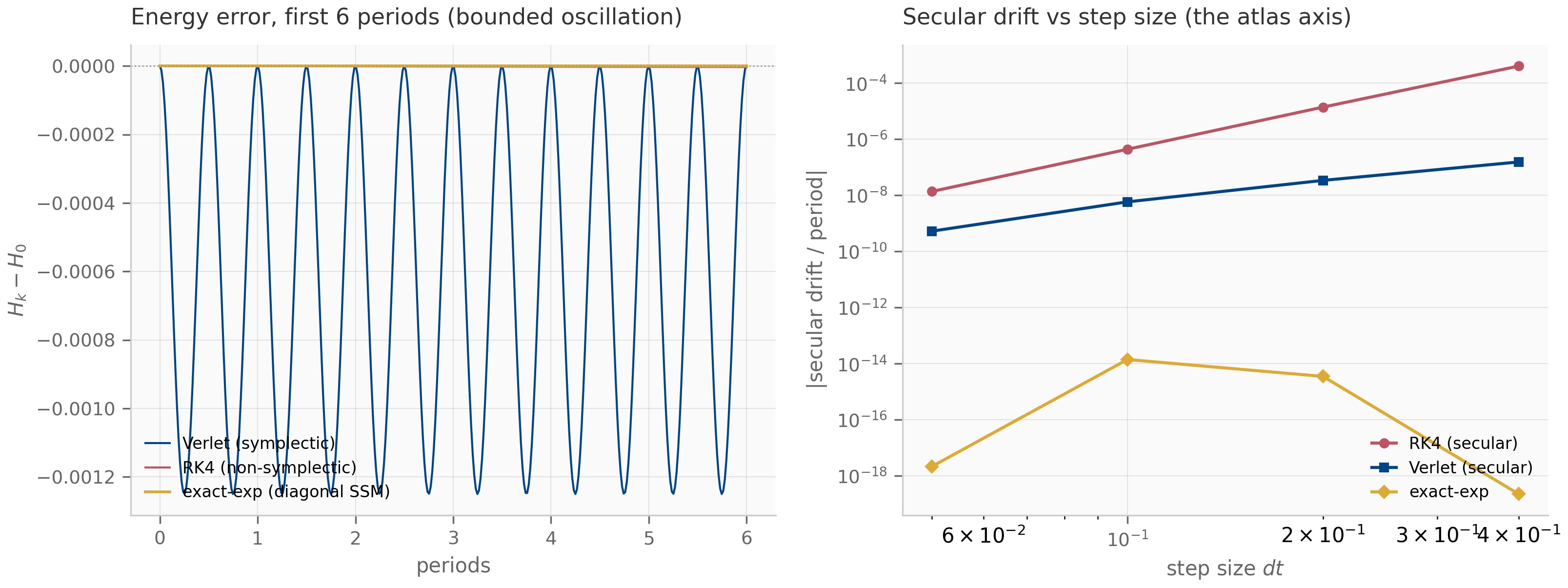
The reading is sharp, and it is the C1 pilot’s premise in miniature. A symplectic integrator (Verlet) buys zero secular energy drift at the cost of a larger bounded oscillation; a non-symplectic one (RK4) has a smaller oscillation but accumulates drift. But the diagonal SSM’s exact exponential dominates both — it has neither drift nor oscillation, because exponentiating a purely imaginary eigenvalue is exactly energy-preserving. The classical symplectic-versus-standard contest is moot for a diagonal SSM. This is not a null result for C1 — it sharpens the pilot’s target: the symplectic advantage can only reappear where the exponential is not applied exactly — a coupled or non-normal transition (the matrix memories of Proposition 13.1), or the forced integral handled at finite order. Whether a trained selective SSM drifts off the diagonal far enough for that to matter is exactly the empirical question the C1 pilot’s symplectic atlas pursues on real matrices — and which this idealized cell cannot answer, only frame. The pilot’s code and findings live in the predecessor repository’s C1 kickoff.

17.3 B — two-timescale benchmarks, and a disentanglement pipeline

The B pilot asks whether an architecture separates a fast process (token bigrams) from a slow one (regime drift). Chapter 14 built the two-timescale HMM and its matched-decay optimality (Theorem 14.4, Theorem 14.1); Chapter 16 built the probing protocol and the paired-comparison statistics (Proposition 16.1, Proposition 16.2); Chapter 15 built the diagnostics, including effective state size (Proposition 15.3). Each measured one facet. The integration runs all three end-to-end on the same reference instance and asks whether the facets cohere.

For each idealized predictor on the known HMM, the pipeline computes three numbers: the effective state size of its regime-propagation operator (Chapter 15, the participation ratio of the operator’s spectrum), its regime-recovery probe accuracy (Chapter 16, a held-out ridge probe of the true regime from the predictor’s carried state), and its predictive cross-entropy (Chapter 14).

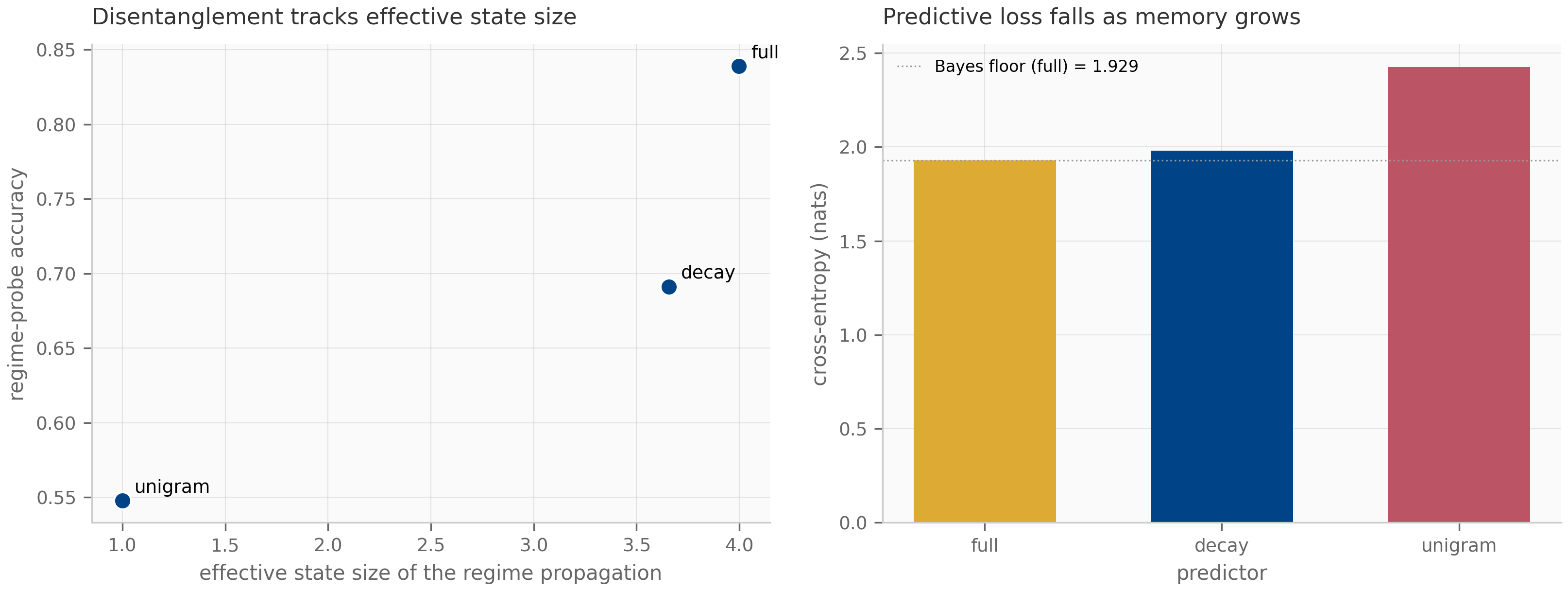
The three instruments cohere: a predictor’s effective state size, its disentanglement, and its loss move together.

Every predictor here is an exact idealization on a known HMM — there is no trained model and no fitted probe target beyond the closed-form filters. The pilot’s contribution is to run this same pipeline on trained checkpoints: probe a real layer’s regime recovery against its measured effective state size, and read its disentanglement against the impossibility ceiling (Proposition 15.1). That program — generators, baselines, the harness — lives in the B kickoff.

17.4 The 13-niche portfolio and the decision rubric

C1 and B are two cells of a larger catalog. The curriculum was designed against a 13-niche portfolio — research directions a numerical-analyst’s reading of sequence models opens up — grouped into four families. The table below maps each niche to representative chapters it draws on as shipped (the author’s reading of the finished book — not the design-time dependency matrix, which together with the full taxonomy and per-niche kickoffs lives in the predecessor’s curriculum design and niche decision).

| Family | Niche | One line | Draws on | Status | |---|---|---|---|---| | A (diagnostics) | A1 Discretization atlas | catalog integrators against SSMs and step sizes | Ch 4–6, 10 | portfolio | | | A2 Update-rules-as-integrators | delta-rule updates as ODE solvers | Ch 6, 12 | portfolio | | | A3 Diagnostics toolkit | Lyapunov spectra + effective state size on trained models | Ch 2, 15 | portfolio | | | A4 Multi-signal regime detection | combine signals to localize regime boundaries | Ch 9, 15 | portfolio | | | A5 Gather-and-Aggregate | the head-importance mechanism behind the recall gap | Ch 14, 15 | portfolio | | B (benchmarks) | B Two-timescale benchmarks | disentangle fast from slow; the §17.3 pipeline | Ch 12, 14, 15, 16 | active (parallel pilot) | | C (NA core) | C1 Symplectic integrators | structure-preserving discretization; the §17.2 atlas | Ch 1–3, 6, 10 | active (primary pilot) | | | C2 Stiffness analysis | is the stiff regime the real training issue? | Ch 5, 6 | portfolio | | | C3 Krylov / matrix-free | the SSD scan as a Krylov target | Ch 3, 9 | portfolio | | | C4 HiPPO conditioning | conditioning of the HiPPO construction | Ch 3, 7 | portfolio | | D (theory) | D1 Reachability | control-theoretic reachability of SSM states | Ch 1, 2 | portfolio | | | D2 Spectral biographies | eigenvalue trajectories across training | Ch 2, 13, 15 | portfolio | | | D3 ODE-solver-as-architecture | architectures named by their integrator | Ch 5, 6, 10 | portfolio |

The two active pilots were not chosen by enumerating value; they were chosen by a decision rubric worth stating, because it generalizes. (i) Direct-transfer depth — C1 is the same symplectic mathematics the author already knows, on a new object, not a loose analogy. (ii) A shared publishing window — A1, C1, and C2 all bear on the exp-trapezoidal integrator and share the Mamba-3 window, so picking any one keeps the family alive. (iii) Non-overlapping machinery — C1 (geometric integration) and B (singular perturbation) use disjoint tools, so they run in parallel without competing for the same hours. (iv) Paid-up-front cost and a documented-null fallback — C1 ships a structural-classification result even if its empirical case returns negative.

17.5 What the lens earned, and its limits

So: did the dynamical-systems lens earn its keep? The honest answer is provisionally yes, and here is exactly how far the evidence reaches.

What it earned is the questions, posed precisely and instrumented. “Is exp-trapezoidal leaving Hamiltonian structure on the table?” is not a question the architecture literature asks; it is natural only once an SSM mode is a discretized ODE and the integrator is a choice with a conservation budget (§17.2). “Does effective state size govern disentanglement?” is measurable only once the state has a spectrum and a participation ratio (§17.3). The lens turned vague intuitions — “Mamba is unstable at long horizons”, “hybrids recall better” — into quantities with diagnostics: Lyapunov exponents (Proposition 15.2), effective state size, the probe signature.

What it has not earned, and cannot from this chapter, is an empirical verdict. Every number here is from an idealized system; the trained-model evidence is the pilots’ forthcoming work. And two limits bound even that future evidence. The first is the cited ceiling: the $\mathsf{TC}^0$ circuit-class impossibility ( Merrill et al. (2024) ; the book’s own counting bound, Proposition 15.1, is its weaker, architecture-agnostic shadow) means no amount of clever discretization or benchmarking lets a fixed-state recurrence do what the complexity class forbids — the pilots can measure where a model sits beneath the ceiling, never move it. The second is mechanistic: the Gather-and-Aggregate finding ( Bick et al. (2025) ) says the recall gap lives in a few attention heads, so a pure-SSM pilot result is read against a known mechanism, not in a vacuum. The lens is an instrument for locating a model in a landscape whose boundaries other tools drew; that is a real contribution, and a bounded one.

17.6 Where this goes

This is the last chapter, so “what’s next” is not more curriculum — it is the research the curriculum exists to enable. The two pilots execute on their own timelines: C1 builds the symplectic atlas on trained Mamba-3 matrices and negative-eigenvalue SSM extensions; B runs the §17.3 pipeline on trained hybrids and reports the disentanglement signature against the ceiling. Both are tracked in the predecessor repository, and both have a documented-null fallback so they produce an artifact either way. The other eleven niches wait in the portfolio with their prerequisites in hand.

With this chapter the book is content-complete: seventeen chapters from linear ODEs to a research program, every architecture read as a dynamical system. The remaining work is not authoring but upkeep — the ordinary maintenance of a living book, its open items tracked in the repository’s issues.

17.7 Exercises

Exercise 17.1 (short)

A constructed SSM mode has eigenvalue $\lambda = -\gamma + i\omega$ with $\gamma > 0$ small. Using §17.2, which integrator — exact-exponential, Verlet, or RK4 — best preserves the mode’s long-horizon energy decay rate, and why does the answer change if the mode is embedded in a coupled (non-diagonalizable) transition?

Exercise 17.2 (short, code)

Run companions/ch17/jax/b_integration.py. Report the effective state size, probe accuracy, and cross-entropy for the full / decay / unigram predictors, and the paired decay-vs-full standard error. What does $\mathrm{SE}_{\text{paired}} \ll \mathrm{SE}_{\text{unpaired}}$ tell you here?

Exercise 17.3 (short)

Pick a portfolio niche from §17.4 — say A3 (diagnostics toolkit) or D2 (spectral biographies). List the chapters it draws on and name the specific companion instruments you would compose to bootstrap it.

Exercise 17.4 (theory) — solution in §17.8

Make the §17.2 bridge precise. Show that the harmonic oscillator $\dot q = p,\ \dot p = -q$ in the complex coordinate $z = q + ip$ satisfies $\dot z = -iz$, that the exact discrete transition over a step $dt$ has magnitude $1$, and conclude that a diagonal SSM with a purely imaginary eigenvalue conserves the mode energy under the exact exponential. Then argue when a symplectic integrator is nonetheless needed.

Exercise 17.5 (theory) — solution in §17.8

Design a two-timescale evaluation for a given pair of architectures, respecting Chapter 16’s discipline: size the task to the discriminative regime (Proposition 16.1), use the distractor rule, and use paired statistics. State precisely what measured outcome would count as a resolved disentanglement difference between the two architectures, and why an unpaired comparison could miss it.

Exercise 17.6 (theory) — solution in §17.8

Argue from the capacity bound (Proposition 15.1) what the C1 and B pilots can and cannot hope to demonstrate. Specifically: can either pilot’s empirical win raise a fixed-state model’s expressive ceiling, or only locate the model beneath it? Frame the answer in terms of the cited-versus-demonstrated boundary of §17.1.

17.8 Full solutions to theory exercises

Solution to Exercise 17.4

Write $z = q + ip$. Then $\dot z = \dot q + i\dot p = p + i(-q) = p - iq$. Factor: $-iz = -i(q + ip) = -iq + p = p - iq$, so $\dot z = -iz$ exactly. The continuous solution is $z(t) = e^{-it}z(0)$, and the exact discrete transition over a step $dt$ is multiplication by $e^{-i\,dt}$, whose magnitude is $|e^{-i\,dt}| = 1$. The mode energy is $H = \tfrac12|z|^2 = \tfrac12(q^2 + p^2)$, and since $|z_k| = |e^{-i\,dt}|^k |z_0| = |z_0|$, the energy is constant for all $k$ — conserved exactly, with no oscillation and no drift (the companion measures a band of $2.8\times10^{-12}$, i.e. machine precision). A diagonal SSM applies $e^{\lambda dt}$ mode-by-mode, so it inherits this exactness on every imaginary mode; the symplectic machinery of Chapter 6 buys nothing it does not already have. A symplectic integrator is needed only when the exponential is not applied exactly: a non-normal or coupled transition (where diagonalization is unavailable or ill-conditioned, Proposition 13.1), or the forced/input integral handled at finite order (Theorem 10.1), where a structure-preserving step can keep the conservation budget a generic step spends. $\blacksquare$

Solution to Exercise 17.5

Size the task so the load sits in the discriminative regime of Proposition 16.1: the two architectures must differ in the capacity the task probes, or the benchmark measures nothing about them (a knee-region requirement, the §16.2 lesson). Construct the separation with the distractor rule — pad with content (fresher competing writes), not neutral fillers, since neutral padding is provably inert under an argmax read-out. Score each architecture’s per-item predictive loss (or probe accuracy) on the same sampled sequences, and compute the paired statistics of Proposition 16.2. A resolved difference is one whose paired confidence interval $\text{mean diff} \pm z\,\mathrm{SE}_{\text{paired}}$ excludes zero. An unpaired comparison can miss it because the per-sequence difficulty is shared (both architectures find the same sequences hard), inflating $\mathrm{SE}_{\text{unpaired}}$ by the shared-difficulty variance that pairing removes — as in §17.3, where the same gap is marginal unpaired and decisive paired. One must also pre-register the suite and avoid post-hoc subset selection, or the selection inflation of Proposition 16.3 manufactures a difference. $\blacksquare$

Solution to Exercise 17.6

Neither pilot can raise the ceiling. The capacity bound (Proposition 15.1) and the cited $\mathsf{TC}^0$ impossibility ( Merrill et al. (2024) ) are statements about every fixed-state recurrence: they bound what such a model can compute regardless of how it is discretized (C1) or benchmarked (B). A better integrator changes the numerical fidelity of the discretization, not the model’s expressive class; a better benchmark changes what we can measure, not what the model can do. So a C1 empirical win means “a structure-preserving integrator tracks this trained mode’s dynamics with less drift”, and a B win means “this architecture’s effective state size lets it disentangle to this measured degree” — both locate the model beneath the ceiling, with higher resolution than before. That is exactly the cited-versus-demonstrated boundary of §17.1: the ceiling is cited (a theorem of others, about a complexity class), and the pilots demonstrate position beneath it (measurements, on trained models). Confusing the two — claiming an integrator or a benchmark “breaks” an impossibility result — is the error the boundary exists to prevent. $\blacksquare$

17.9 Companion code

The companions live in companions/ch17/{jax,julia} and are float64 throughout; they compose shipped instruments rather than introduce new kernels, so there is no torch port (it would only re-run the JAX modules). Each produces a new integrated signature; the component values reduce to the originating chapters’ (pinned in the tests).

• jax/c1_integration.py — the C1 atlas cell (§17.2). Composes Chapter 6’s symplectic/RK4 steppers and Chapter 10’s complex-mode recurrence to compare the long-horizon energy conservation of the exact-exponential, Verlet, and RK4 integrators on a harmonic-oscillator SSM mode. The reused RK4 path reproduces Chapter 6’s rk4_drift_per_period exactly. Produces c1-atlas-cell.png.
• jax/b_integration.py — the B disentanglement pipeline (§17.3). Composes Chapter 14’s HMM and idealized predictors, Chapter 16’s probe signature and paired comparison, and Chapter 15’s effective state size into one readout linking effective state size, probe accuracy, and loss across the predictor family. Produces b-disentanglement.png.
• julia/symplectic_crosscheck.jl — a stdlib-only, independent-language cross-check of the C1 atlas cell (the C1 pilot’s atlas is itself Julia), matching the JAX energy-conservation signatures to $< 10^{-9}$.

PYTHONPATH=. python companions/ch17/jax/c1_integration.py
PYTHONPATH=. python companions/ch17/jax/b_integration.py
make companion-jax-tests          # all chapters' JAX suites
julia --project=companions/ch17/julia companions/ch17/julia/runtests.jl