Delta-rule lineage: DeltaNet, Gated DeltaNet, Kimi Linear

12.1 The recall objective and its gradient flow

Chapter 11 ended at a wall (Proposition 11.4): the additive state $S = \sum_i \phi(k_i)v_i^\top$ accumulates and never forgets, so every stored pair interferes with every retrieval through the key overlaps $k_i^\top k_j$, and no finite state escapes the trend. The closing promise was a smarter write rule. To derive one, stop postulating recurrences and instead ask what the state is for.

The state of every architecture in this part of the book is an associative memory: it should return $v$ when probed with $k$. Make that a loss. At time $t$, with the incoming pair $(k_t, v_t)$,

Two conventions before anything else. First, shapes: this chapter writes the state as $S \in \mathbb{R}^{d_v \times d_k}$ with retrieval $S k$ — the row-state form used by the DeltaNet literature and by Chapter 3’s low-rank update discussion. Chapter 11 wrote the transposed form ($S \in \mathbb{R}^{d_k \times d_v}$, projector acting on the left); the map $S \mapsto S^\top$ converts one to the other, and every claim below transposes with it. Second, the feature map: the delta-rule literature works with the keys directly (typically $\ell_2$-normalized) rather than through a kernel feature map $\phi$; we follow that and write $k_t$ for what Chapter 11 would call $\phi(k_t)$. Nothing in this chapter depends on the distinction — and the normalization choice will turn out to be a stability decision (§12.4).

Gradient descent on $\mathcal{L}_t$ in continuous time is the recall gradient flow

a linear (affine) matrix ODE. Its equilibrium is the rank-one matrix that retrieves perfectly:

The proof is a two-line computation with the substitution $E = S - S^\star$ (Exercise 12.5 carries it through the discretizations). The inert orthogonal complement is a feature, not a defect — it is persistent memory, and §12.6 will need a gate precisely because gradient flow on the current pair never cleans up stale directions on its own.

Everything in this chapter is now one sentence: DeltaNet, Longhorn, and their gated descendants are different one-step discretizations of this flow, interleaved over a stream of pairs $(k_t, v_t)$. The architecture zoo becomes an integrator catalog, and the book’s Part-I machinery applies.

12.2 DeltaNet: one explicit gradient step

Take one forward-Euler step of size $\beta_t$ on the recall flow (Chapter 4’s explicit workhorse), at the incoming pair:

The identity is one distribution of terms: $S_{t-1}(I - \beta k k^\top) + \beta v k^\top = S_{t-1} + \beta(v - S_{t-1}k)k^\top$. Chapter 3 previewed exactly this update as the recurring “low-rank correction” pattern — for $\beta_t \|k_t\|^2 < 1$ the factor $(I - \beta_t k_t k_t^\top)$ is a contraction toward the hyperplane $k_t^\perp$, and at $\beta_t \|k_t\|^2 = 1$ it is the orthogonal projector onto it. With $\beta_t \in (0,1]$ a learned, input-dependent write strength and the read $o_t = S_t q_t$, this recurrence is DeltaNet’s state update Yang et al. (2024) , the delta rule of fast-weight programming Schlag et al. (2021) made into a sequence layer. The companion’s lax.scan (rank-one form) and a deliberately different materialized-projector loop agree to $1.8 \times 10^{-15}$ over 48 steps — the two faces are one operator.

What did the erase term buy over Chapter 11’s accumulation? The defining semantics: re-storing a key replaces its value. Write $(k, v_1)$, then $(k, v_2)$, with $\beta = 1$ on a unit key. The erase factor annihilates the old binding before the new write lands, so the delta-rule state retrieves $S k = v_2$ exactly — measured residual $4.4 \times 10^{-16}$ — while the additive state retrieves $v_1 + v_2$, off by the entire stale residue (measured $\ell_\infty$ error $1.27$ on the same data). An additive memory can only pile bindings on top of each other; a delta-rule memory updates them.

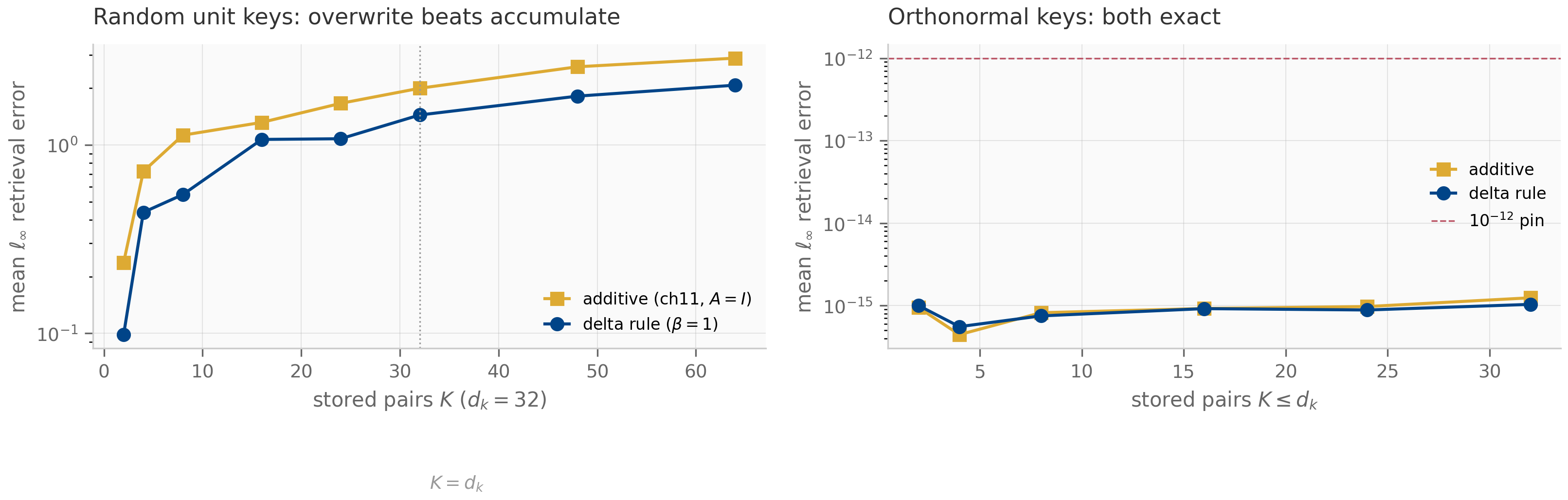
The figure is deliberately honest about the limit. With orthonormal keys both rules are exact — the delta rule’s advantage is zero when keys do not overlap — and with random keys both error curves still grow as $K$ passes $d_k$: a rank-$d_k$ state cannot hold more than $d_k$ independent associations no matter how cleverly it writes (Proposition 11.4 still binds). The delta rule answers Chapter 11’s interference problem and its staleness problem (the overwrite), not the capacity bound. That distinction is exactly where Chapter 13’s matrix-memory architectures and Chapter 14’s hybrids will pick up.

12.3 Longhorn: the implicit step

Forward Euler is not the only one-step method, and Chapter 6 taught the alternative. Longhorn Liu et al. (2024) reaches it from the optimization side: frame the update as amortized online learning and solve, at each step, the regularized problem

a trust-region (proximal) step: improve recall on the incoming pair, but do not move far from the state you have. Setting the gradient to zero gives

Read the right-hand form against §12.1: this is the recall gradient evaluated at the endpoint $S_t$, with step size $h = 1/\alpha_t$ — the backward-Euler step on the recall flow, the implicit method of Chapter 6.

An implicit equation usually costs a solve. Here the solve is free:

The proof (Exercise 12.4, §12.9) is the classic implicit-solve move: right- multiply the stationarity equation by $k_t$, solve the resulting scalar equation for the post-update prediction $S_t k_t$, and substitute back. In the companion the identification is structural — longhorn_step simply is delta_rule_step evaluated at $\beta^{\mathrm{eff}}$ — so the closed form gets an independent certificate instead: solving the stationarity system $S_t(\alpha I + k k^\top) = \alpha S_{t-1} + v k^\top$ by dense linear solve (no code shared with the rank-one form) reproduces it to $4.4 \times 10^{-16}$, and the closed form zeroes the stationarity residual to $7.8 \times 10^{-16}$ (pinned $< 10^{-12}$ in tests/test_longhorn.py::test_closed_form_equals_dense_implicit_solve). Explicit and implicit methods on this flow live in the same parametric family — they differ only in how the effective step size responds to the data. DeltaNet’s $\beta_t$ is whatever the network learned to emit; Longhorn’s $\beta_t^{\mathrm{eff}}$ self-adapts to the key magnitude. Scaling the key by $10^2$ pushes the product $\beta^{\mathrm{eff}}\|k\|^2$ to $1 - 1.7\times 10^{-5}$; by $10^4$, to $1 - 1.7\times 10^{-9}$ — approaching but provably never reaching $1$. That denominator is the entire difference between the two architectures, and §12.4 shows it is exactly the difference between conditional and unconditional stability.

12.4 Stability regions: the explicit/implicit dichotomy

Both updates iterate an affine map in $S$, so no linearization is needed: with $S^\star = v k^\top / \|k\|^2$ and $E_t = S_t - S^\star$, a step at the (for now, repeated) pair $(k, v)$ gives exactly

The iteration matrix is a rank-one perturbation of the identity; its spectrum is immediate.

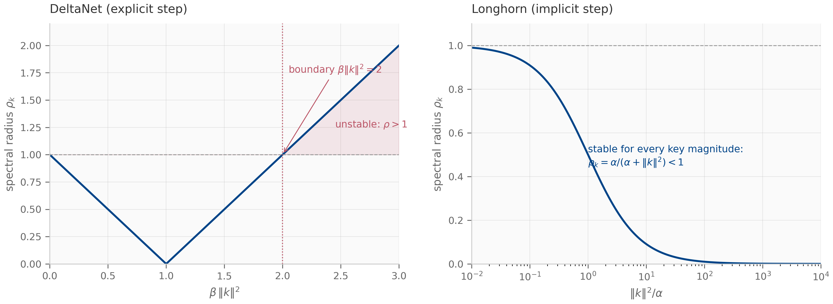
Because the deviation recurrence is exact — not a linearization — the geometric law is measurable to machine precision. Starting from $S_0 = 0$ under a repeated unit-norm key, the per-step ratio $\|E_t\|_F / \|E_{t-1}\|_F$ measured from the companion equals the analytic radius to twelve digits: $1.500000000000$ for DeltaNet at $\beta\|k\|^2 = 2.5$, $0.500000000000$ for Longhorn at $\alpha = \|k\|^2$. The trajectories make the dichotomy visceral:

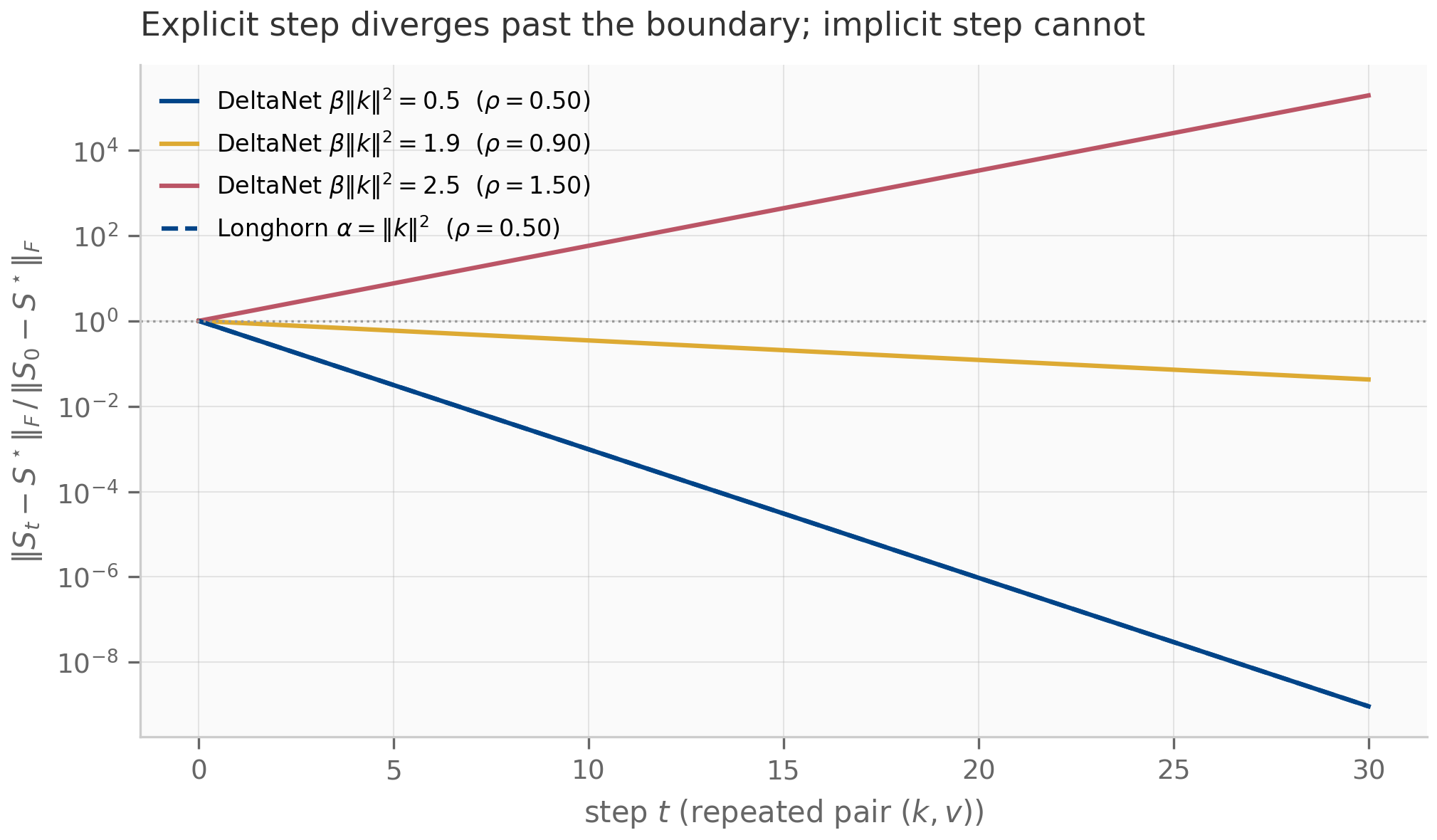
One degenerate-looking feature of Theorem 12.4 deserves emphasis: the orthogonal eigenvalue is exactly $1$ for both methods. Neither integrator forgets directions it has not been asked about — stability here is about the write direction only. Whole-state forgetting needs a different mechanism (§12.6).

Why trained DeltaNets are stable anyway. The dichotomy explains a design detail that looks cosmetic in the paper and is load-bearing in the lens: Yang et al. $\ell_2$-normalize keys and parameterize $\beta_t = \mathrm{sigmoid}(\cdot) \in (0,1)$ Yang et al. (2024) . With $\|k_t\| = 1$ that pins $\beta_t\|k_t\|^2 < 1$ — not merely inside the stability interval $(0,2)$ but inside its monotonically-contracting half. And the per-step guarantee composes, which discharges the repeated-pair scoping above: with $\beta_t\|k_t\|^2 < 1$ every factor $I - \beta_t k_t k_t^\top$ has eigenvalues in $(0, 1]$, so the streaming product over any key sequence is non-expansive — the repeated pair is the worst case, not a special case. The architecture’s normalization choices are its stability guarantee, chosen at design time the way a step-size rule is chosen for an integrator. Longhorn needs no such guard, and that is precisely its selling point: stability by method, not by parameterization — the implicit-method trade Chapter 6 priced out, here with a free solve.

12.5 Chunkwise parallelization: the WY trick

The recurrent delta rule is $O(\seqlen)$ sequential — fine for inference, hostile to training hardware. Chapter 11 met the same tension and resolved it with a second face of the same operator (Theorem 11.1); the delta rule’s resolution is the same move with one extra piece of numerical linear algebra. Split the sequence into chunks of size $C$ and unroll the erase-then-write form across one chunk:

with $R$ the chunk’s accumulated writes — the chunk’s own §12.2 recurrence run from a zero entry state, which is exactly how the companion materializes it. The cross-chunk recurrence is now one affine update per chunk ($\seqlen/C$ sequential steps) and everything inside a chunk touches only chunk-local data Yang et al. (2024) . The remaining cost is the erase product $P$ — naively a chain of $d_k \times d_k$ matrix products. But $P$ is a product of rank-one perturbations of $I$, and numerical linear algebra has compressed exactly this object for decades:

The induction (Exercise 12.6, §12.9) is three lines. The companion pins both identities at machine precision on a stable-regime stream (unit-norm keys, $\beta_t < 1$ — §12.4’s recommended operating point): the WY form matches the explicitly multiplied product to $3.7 \times 10^{-16}$ at worst across chunk sizes $C = 2$ through $64$, and the chunkwise driver — cross-chunk state passing with chunk-local sweeps — reproduces the monolithic recurrence bitwise (measured difference $0.0$ for every chunk size $C \mid \seqlen$, because both run the same scan arithmetic in the same order). As in Chapter 11, the equivalence is the correctness certificate for the production form: one operator, two computation schedules.

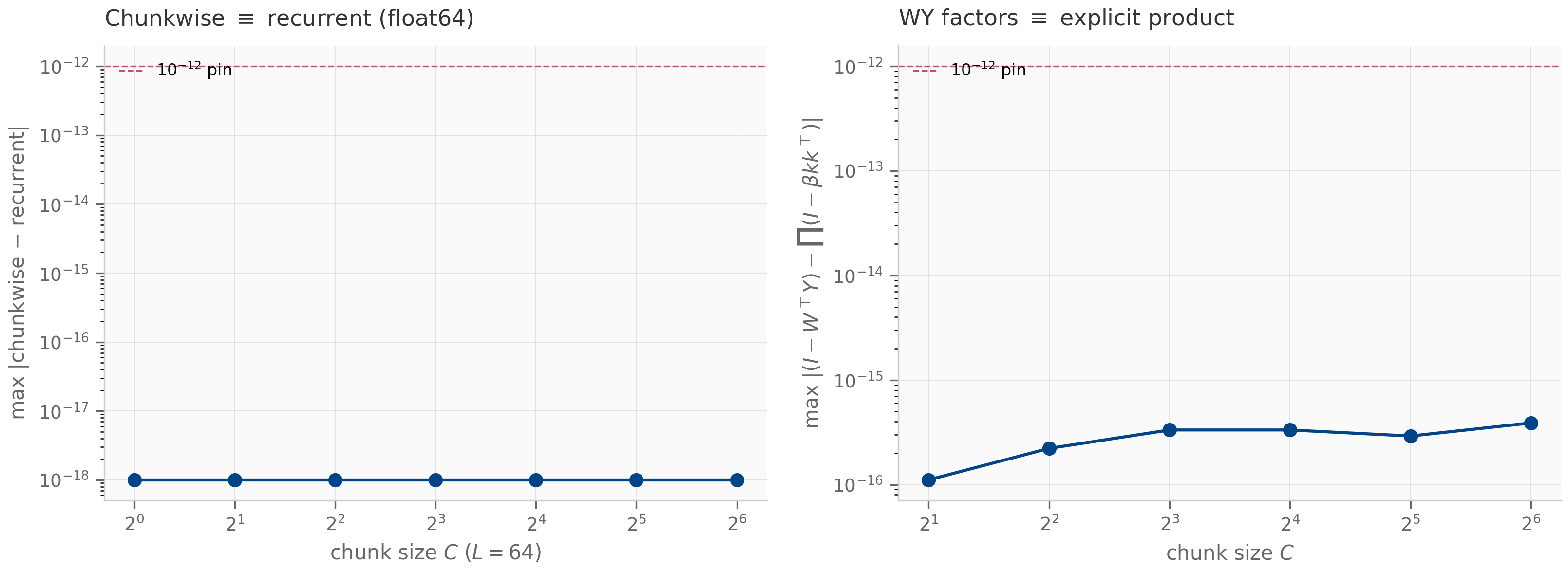
The practical punchline mirrors Chapter 11’s: the recurrent form is the inference mode, the chunkwise form is the training mode, and a fused kernel is an engineering refinement of an identity that is already exact in pure JAX.

12.6 Gating the delta rule: Gated DeltaNet and Kimi Linear

Theorem 12.4 left one direction untouched: everything orthogonal to the current key sits at eigenvalue exactly $1$. A delta-rule memory never spontaneously forgets — stale bindings persist until their key is revisited. Chapter 9’s selective SSMs had the complementary skill: a scalar decay $\discA_t$ that forgets everything, uniformly. Gated DeltaNet Yang et al. (2025) composes the two:

The gate multiplies the erased state; the fresh write lands ungated. Both parents are exact limits, and the companion pins both reductions: $\gamma_t \equiv 1$ recovers plain DeltaNet to $1.8 \times 10^{-15}$, and $\beta_t \equiv 0$ is pure exponential decay $S_t = \gamma_t S_{t-1}$ — Chapter 9’s scalar-decay contraction with the carry promoted to a matrix, the same promotion Chapter 11 made for accumulation (Theorem 11.2).

The division of labor is exact, not approximate. Store a pair $(k_A, v_A)$, then perform $T$ gated-delta writes whose keys are orthogonal to $k_A$: the erase factors never touch the $k_A$ direction, so the retrieval decays only through the gate,

and the companion measures the product law at $5.6 \times 10^{-17}$ over forty writes. Gating forgets uniformly (a half-life for everything); the delta rule forgets selectively (exact overwrite of what is re-keyed). An architecture with both has independent control of the two timescales — which is why this update, not the plain delta rule, is what shipped. And the gate does not cost trainability: extending §12.5’s chunkwise/WY machinery to the $\gamma$-decayed erase product is a core contribution of the Gated DeltaNet paper Yang et al. (2025) , so the gated update trains with the same hardware efficiency.

That shipping lineage is current production history, summarized at architecture level. Kimi Linear Kimi Team (2025) builds its KDA (Kimi Delta Attention) layer as a refinement of exactly this gated update — the scalar $\gamma_t$ replaced by per-channel diagonal gates, a finer-grained forgetting clock — and interleaves KDA with full attention at a 3:1 layer ratio, reporting up to a 75% KV-cache reduction at million-token contexts. As of mid-2026 this family — the gated delta rule adopted as the linear layer of public hybrid stacks, KDA in the Kimi Linear release — is the delta rule’s production form. This book derives the update those systems share; their layer-ratio and gate-granularity choices belong to Chapter 14’s hybrid design space, and the chapter makes no derived claims about KDA beyond the gated update above.

Step back to see the family whole. Chapter 9 proved selective SSMs and masked attention are one object (Theorem 9.5); Chapter 11 added the accumulation face; this chapter added the write-rule axis: accumulate ($\beta$-write only), erase-and-write (delta), decay-erase-write (gated delta) — each one discretization choice on the same recall flow. Two limits now bracket the design space: the pure-decay limit ($\beta \to 0$, an SSM forgetting on a slow clock) and the pure-write limit (attention-like immediate binding). Pilot B’s two-timescale benchmarks live exactly in that bracket — attention as the fast boundary layer, the decaying state as the slow manifold — and Chapters 14 and 16 build the architectures and the measurement protocol for it.

12.7 What’s next

This chapter closed Chapter 9’s “delta-rule lineage” promise and Chapter 11’s capacity hand-off: the write rule is now an optimizer step, and its stability theory is Chapters 5–6 applied to a new flow.

Two threads leave here open by design. Chapter 13 takes the lineage’s next generalization: RWKV-7’s generalized delta rule (transition $\mathrm{diag} +$ rank-one in a learned direction, not the key itself) and xLSTM’s matrix memory with exponential gating — the gate moved inside the nonlinearity, with its own stabilization problem. Chapter 14 mixes these layers with attention into the production hybrids named above, where the layer-ratio and gate-granularity decisions we deferred become the design variables; Chapter 16 then builds the evaluation methodology — including the two-timescale protocol pilot B contributes — that makes the comparisons honest.

12.8 Exercises

Three short problems (solutions inline) and three longer ones (solutions in §12.9).

Exercise 12.1 (short)

With $d_k = d_v = 2$, unit key $k = (1, 0)^\top$, and values $v_1 = (1, 2)^\top$, $v_2 = (3, -1)^\top$: compute the delta-rule state after writing $(k, v_1)$ then $(k, v_2)$ with $\beta = 1$, and the additive state $\sum_i v_i k^\top$ for the same writes. Verify the retrievals $S k$ are $v_2$ and $v_1 + v_2$ respectively.

Exercise 12.2 (short, code)

Run companions/ch12/jax/delta_rule.py. Report the overwrite residuals and the $K = 32$ recall errors, then explain in one sentence why the orthonormal-key panel shows both rules exact.

Exercise 12.3 (short)

For $\alpha = 1$ and $\|k\|^2 \in \{1, 4, 100\}$, compute Longhorn’s $\beta^{\mathrm{eff}}$, the product $\beta^{\mathrm{eff}}\|k\|^2$, and the radius $\rho_k$. Verify the complement identity $\rho_k + \beta^{\mathrm{eff}}\|k\|^2 = 1$ and state what it says about where the “stable mass” goes as keys grow.

Exercise 12.4 (theory) — solution in §12.9

Derive Theorem 12.3: starting from the stationarity equation $\alpha(S_t - S_{t-1}) + (S_t k - v)k^\top = 0$, obtain the closed form by solving for the post-update prediction $S_t k$ first. Where exactly does $\alpha > 0$ get used?

Exercise 12.5 (theory) — solution in §12.9

Prove Theorem 12.4: compute the full spectrum of $I - \beta^{\mathrm{eff}} kk^\top$, derive the deviation recurrence $E_t = E_{t-1}(I - \beta^{\mathrm{eff}} kk^\top)$ from either update, and conclude the stability characterizations for both step-size rules. Explain why starting from $S_0 = 0$ makes $\|E_t\|_F$ exactly geometric rather than merely asymptotically so.

Exercise 12.6 (theory) — solution in §12.9

Prove Theorem 12.5 by induction on the chunk position, and count the cost of applying $P$ to a $d_v \times d_k$ state via the WY form versus the materialized product, for chunk size $C \ll d_k$.

12.9 Full solutions to theory exercises

Solution to Exercise 12.4

Right-multiply the stationarity equation by $k$:

a scalar-shaped linear equation for the vector $p := S_t k$ (the matrix unknown has collapsed because only $S_t k$ appears). Since $\alpha > 0$ the coefficient $\alpha + \|k\|^2$ is strictly positive — this is the only place positivity is needed, and it is what makes the implicit solve nonsingular for every key, including $k = 0$. Solve:

Substitute into the stationarity equation rearranged as $S_t = S_{t-1} + \tfrac{1}{\alpha}(v - S_t k)k^\top$:

Solution to Exercise 12.5

Spectrum. For any unit vector $u \perp k$: $(I - \beta^{\mathrm{eff}} kk^\top)u = u$, giving eigenvalue $1$ with multiplicity $d_k - 1$. For $u = k/\|k\|$: $(I - \beta^{\mathrm{eff}} kk^\top)k = (1 - \beta^{\mathrm{eff}} \|k\|^2)k$, the single non-unit eigenvalue.

Deviation recurrence. Both updates have the form $S_t = S_{t-1} + \beta^{\mathrm{eff}}(v - S_{t-1}k)k^\top$ (Theorem 12.3 for Longhorn). Since $S^\star k = v$,

The affine parts cancel exactly — no linearization, no remainder.

Characterizations. Deviation components along $k^\perp$ (in the row space) are multiplied by $1$ each step; the component along $k$ is multiplied by $\lambda = 1 - \beta^{\mathrm{eff}}\|k\|^2$. Convergence of the corrected direction requires $|\lambda| < 1$, i.e. $\beta^{\mathrm{eff}}\|k\|^2 \in (0, 2)$. DeltaNet’s free $\beta$ can violate this; Longhorn’s $\beta^{\mathrm{eff}}\|k\|^2 = \|k\|^2/(\alpha + \|k\|^2) \in (0, 1) \subset (0, 2)$ cannot, and $\lambda = \alpha/(\alpha + \|k\|^2) \in (0, 1)$ directly.

Exact geometry from $S_0 = 0$. Then $E_0 = -S^\star = -vk^\top/\|k\|^2$, whose every row is a multiple of $k^\top$: the deviation starts entirely in the contracted direction, with no component on the eigenvalue-$1$ complement. Hence $\|E_t\|_F = |\lambda|^t\,\|E_0\|_F$ exactly — which is why the measured per-step ratios in §12.4 reproduce $\rho$ to twelve digits rather than only in the limit. $\qquad\blacksquare$

Solution to Exercise 12.6

Induction. Base $t = 0$: the empty product is $I = I - 0$, with empty factors. Step: assume $P_{1:t-1} = I - W_{1:t-1}^\top Y_{1:t-1}$ where the rows of $Y_{1:t-1}$ are $k_1, \dots, k_{t-1}$. Then

The correction is rank one with row direction $k_t^\top$, so append $y_t = k_t$ and

which is the stated recursion, and $P_{1:t} = I - W_{1:t}^\top Y_{1:t}$.

Cost. WY application $SP = S - (SW^\top)Y$: one $(d_v \times d_k)(d_k \times C)$ GEMM and one $(d_v \times C)(C \times d_k)$ GEMM, $O(d_v d_k C)$ total, plus the $O(C^2 d_k)$ one-time factor build. The materialized product costs $O(C\,d_k^2)$ to build and $O(d_v d_k^2)$ to apply: for $C \ll d_k$ the WY route wins by a factor $\sim d_k/C$ on both counts, and — the practical point — both of its operations are GEMMs, the shape hardware wants. $\qquad\blacksquare$

12.10 Companion code

The companions live in companions/ch12/{jax,torch,julia} and are float64 throughout. The JAX modules are canonical and produce all four figures; the torch modules mirror the three operator updates with cross-framework parity pinned to $< 10^{-9}$; the Julia module ports the §12.4 stability analysis to a third language using only the standard library, pinning the same closed forms and trajectory ratios.

# JAX (canonical; emits the four figures to public/figures/ch12/)
PYTHONPATH=. python companions/ch12/jax/delta_rule.py
PYTHONPATH=. python companions/ch12/jax/longhorn.py
PYTHONPATH=. python companions/ch12/jax/stability.py
PYTHONPATH=. python companions/ch12/jax/chunkwise.py
PYTHONPATH=. python companions/ch12/jax/gated_delta.py

# Tests: JAX identities (< 1e-12), torch parity (< 1e-9), Julia stability suite
.venv/bin/pytest companions/ch12/jax companions/ch12/torch -q
julia --project=companions/ch12/julia companions/ch12/julia/runtests.jl

• delta_rule.py — the explicit step, its two algebraic faces, the fixed point, overwrite-vs-accumulate semantics, and the recall comparison figure (§12.1–12.2).
• longhorn.py — the implicit step via its closed form, verified against an independent dense solve of the stationarity system, plus the structural identity with the delta rule and the exact geometric error trajectories (§12.3–12.4).
• stability.py — the closed-form spectral radii, the named boundary, and the Rayleigh-quotient drift guard behind the stability-regions figure (§12.4).
• chunkwise.py — the WY representation, its two-GEMM application, and the chunkwise≡recurrent certificate (§12.5).
• gated_delta.py — the gated update, both exact reductions, and the $\gamma^T$ uniform-forgetting law (§12.6). The torch mirror’s test file also documents the buffers-vs-Parameters distinction (a learned rate projection is a Parameter; a fixed rate floor is a buffer).