Counter-evidence and diagnostic tools: where SSMs fail
The prosecution's file — what fixed-state and SSM-heavy designs provably cannot do (the TC⁰ ceiling, the illusion of state, the copying separation) and the diagnostic toolkit that measures stability and capacity on real systems, from an architecture-agnostic information-counting bound through the Benettin–QR Lyapunov estimator and its resolution limit to effective state size as a regime diagnostic, all validated against known ground truth.
On this page
- 15.1 The prosecution’s file
- 15.2 The expressivity ceiling: TC⁰ and the illusion of state
- 15.3 The capacity bound: a counting argument
- 15.4 Lyapunov diagnostics: measuring stability on a concrete system
- 15.5 Regime detection and effective state size
- 15.6 The mechanistic verdict
- 15.7 What’s next
- 15.8 Exercises
- Exercise 15.1 (short)
- Exercise 15.2 (short, code)
- Exercise 15.3 (short, code)
- Exercise 15.4 (theory) — solution in §15.9
- Exercise 15.5 (theory) — solution in §15.9
- Exercise 15.6 (theory) — solution in §15.9
- 15.9 Full solutions to theory exercises
- Solution to Exercise 15.4
- Solution to Exercise 15.5
- Solution to Exercise 15.6
- 15.10 Companion code
Counter-evidence and diagnostic tools: where SSMs fail
15.1 The prosecution’s file
Three earlier chapters filed their counter-evidence here. Chapter 13 closed by naming this chapter “the counter-evidence file: it takes the stability questions raised here — when does a matrix memory’s recurrence stay bounded, and what can it provably not do — and turns them into diagnostics and impossibility results.” Chapter 14 cast it as the prosecution to its own defense of hybrids. Chapter 16 left “the impossibility side of the story — what else fixed state provably cannot do” explicitly to “Chapter 15’s file.” This chapter discharges all three.
The lens the book has used — a sequence layer is a dynamical system, read through its state — obliges two kinds of counter-evidence, and they are different in character:
-
Impossibility. Some tasks are out of reach not for want of tuning but for structural reasons: a fixed-size state is an information bottleneck, and a parallelizable recurrence sits in a circuit-complexity class that excludes genuinely sequential computation. These are theorems about every model of a given shape, and the strongest of them — the ceiling, the copying separation — are deep results we cite and attribute, never re-derive (§15.2). The one impossibility we can prove in a page is a counting bound (§15.3); it is deliberately weaker than the cited theorems, and saying exactly how it is weaker is half its value.
-
Diagnosis. Impossibility says what no such model can do; it does not tell you where this trained model sits. For that you need instruments that measure a concrete recurrence: its stability (does the state stay bounded? — Lyapunov exponents, §15.4) and its usable memory (how many modes actually persist? — effective state size, §15.5). These are the numerical-analyst’s tools, and the discipline of the chapter is to validate each against a system whose answer we know by construction before trusting it on a system we don’t.
The boundary between the two threads is the boundary between cited and proven, and the chapter marks it everywhere: a result in a shaded box with an attribution is someone else’s theorem; a result in a numbered proposition with a proof (or an exercise pointing to one) is ours, and every number it claims is measured by a companion.
15.2 The expressivity ceiling: TC⁰ and the illusion of state
The deepest counter-evidence is complexity-theoretic, and it cuts both ways. A transformer with logarithmic-precision arithmetic and a state-space model are, to first order, in the same computational class — and that class is small.
The phrase “illusion of state” is precise: a recurrence that the associative scan of Chapters 8–9 parallelizes is, by that very parallelizability, confined to the shallow-circuit class. The state buys linear-time inference and a place to put memory; it does not buy sequential expressivity. This is the formal counter-weight to a claim Chapter 13 flagged and deferred: RWKV-7’s paper reports that it “recognizes all regular languages,” apparently reaching above the ceiling. The reconciliation is in the fine print — that result holds for a fixed network with precision and depth allowed to grow with the automaton, not within the uniform, fixed-precision regime the impossibility theorems assume.
The copying separation makes the abstract ceiling concrete. Of Jelassi et al. Jelassi et al. (2024) : a two-layer transformer copies strings of length exponential in its size, while a fixed-state recurrence is bounded by what its state can hold — “structural, not a tuning issue.” That structural bound is the one piece of the impossibility story we can prove ourselves, and §15.3 does.
15.3 The capacity bound: a counting argument
Chapter 11 proved a rank wall for linear attention (Proposition 11.4) and Chapter 16 measured a recall cliff for an exact-capacity slot model (Proposition 16.1). Both are instances of one architecture-agnostic fact: a finite state is a finite communication channel, and no amount of cleverness lets a channel carry more than its capacity.
Let a deterministic sequence model process inputs by a recurrence carrying a hidden state in a set representable in coordinates at bits each, so . Suppose a task requires the model, after reading a prefix, to answer queries whose correct answers differ across a family of prefixes that must be distinguished. If , then two distinct prefixes induce the same post-prefix state, and the model answers them identically — wrong on at least one. In particular, losslessly recalling length- sequences over an alphabet requires
The proof is pure pigeonhole (Exercise 15.4): the post-prefix state is a deterministic function , every later output factors through , and forces a collision. Specializing to verbatim copy, the length- strings must all be distinguished, giving .
Two things make this honest rather than impressive. First, it is weaker than the cited theorems: it bounds lossless recall by counting, where Jelassi et al. exhibit the separation empirically and Merrill et al. place it in a complexity hierarchy. A real model also fails below this bound — interference, finite training, and lossy encodings mean the usable capacity is a fraction of . The counting bound is the ceiling of the ceiling. Second, it is architecture-agnostic: Chapter 11’s rank- state (, with the bits of a stored coordinate) and Chapter 16’s -slot store are the two instances where the abstract becomes concrete, and the chapter derived each separately. Here they are one count.
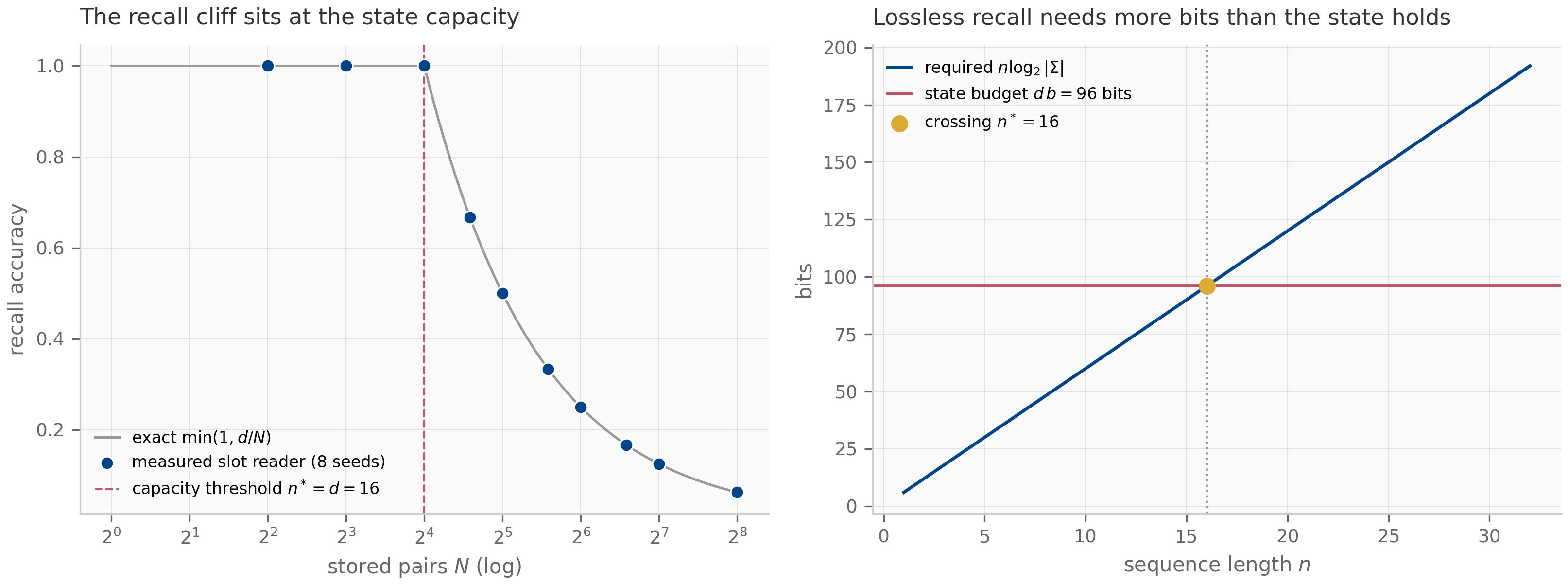
The companion realizes the bound on Chapter 16’s slot model, where each of slots holds one token-pair, i.e. bits. The abstract budget then meets the lossless requirement exactly at , and the measured recall cliff sits there.
15.4 Lyapunov diagnostics: measuring stability on a concrete system
Impossibility is about all models; the rest of the chapter is about this one. The first instrument measures stability. Chapter 2 defined a system’s Lyapunov exponents as the asymptotic log-growth rates of its state (Definition 2.2, Theorem 2.1) and computed them with the Benettin QR algorithm Benettin et al. (1980) ; we reuse that engine unchanged and ask what it can and cannot tell us about a recurrence whose transition we did not choose — a trained-like SSM layer, the matrix memory of Chapter 13, a selective scan.
Let be the per-step Jacobian sequence of a recurrence, and let be the Benettin–QR estimate over a trace of length .
- (Recovery.) If the system is autonomous with a diagonalizable transition , then as ; the estimate is a time average, so its error decays like , and the top exponent (largest spectral gap) converges fastest.
- (Divergence identity.) For any and every , exactly, because the QR triangular factors satisfy . The sum of the exponents is the robust summary that survives even when the individual exponents do not.
- (Resolution limit.) When several modes share a modulus in a non-normal recurrence, the QR frame cannot isolate the individual exponents — they carry splitting noise — though their mean stays pinned by part 2.
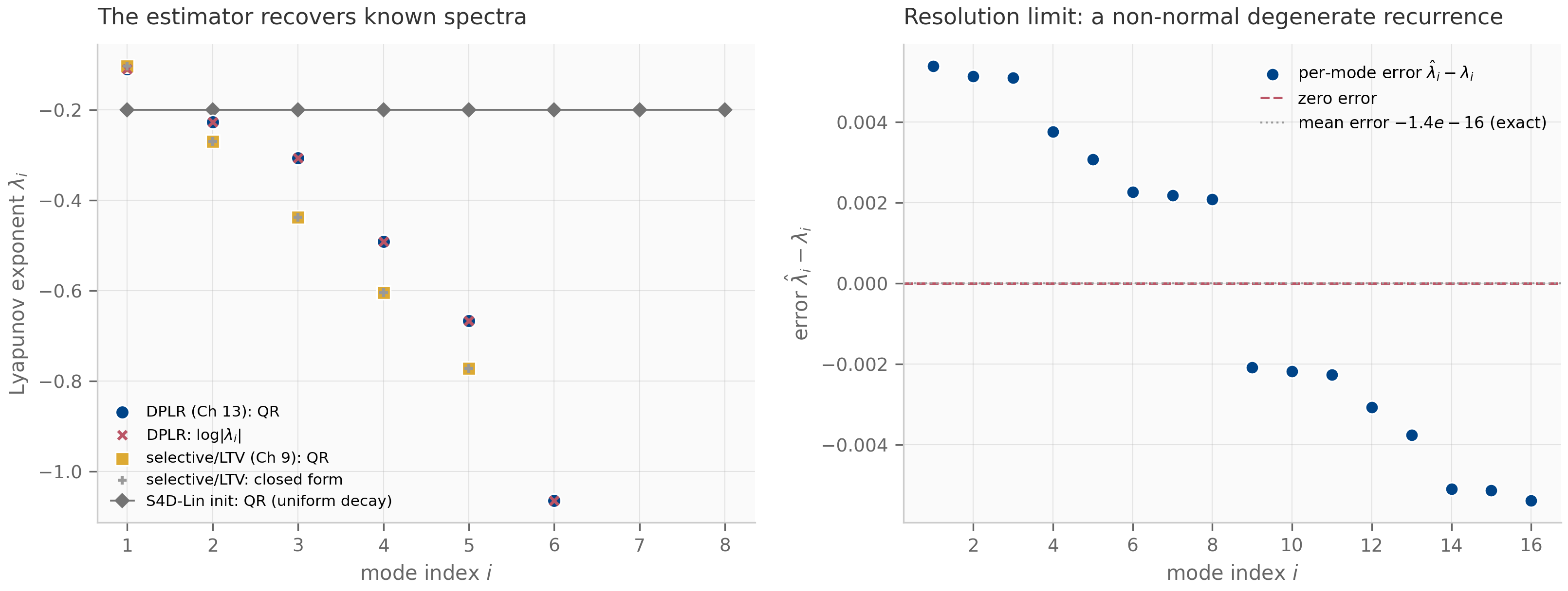
Part 1 is the multiplicative-ergodic / QR-convergence theorem specialized to a constant map; part 2 is exact each step (Exercise 15.5); part 3 is the subtlety that matters in practice, and it is not about degeneracy alone. The companion makes the distinction sharp. A diagonal-plus-rank-one transition from Chapter 13 (Proposition 13.1), symmetric with distinct moduli, is recovered to a measured over steps (top exponent to — fastest, as promised); a diagonal selective/LTV Jacobian stream from Chapter 9 is recovered exactly (the decoupled coordinates make the QR trivial). Even a system that resembles an S4D-Lin layer at initialization — every mode decaying at the same rate , a degenerate spectrum — is recovered exactly, because its modes are decoupled.
The resolution limit appears only when degenerate modes are coupled: Chapter 2’s damped ring, a non-normal recurrence whose modes share a decay rate but rotate at different frequencies, scatters the per-mode estimates by a measured while the mean rate stays exact to . The lesson for diagnosing a trained model is concrete: trust the top exponent and the sum; distrust an individual interior exponent of a coupled system unless its modulus is well separated.
This is the diagnostic Chapter 7 anticipated — “the structure a stability or Lyapunov analysis of a trained S4 layer measures against” (Proposition 7.3) — and the one Chapter 2 named as the unified internal/input–output stability check, since an eigenvalue drifting toward shows up as a Lyapunov exponent crossing zero (Theorem 2.4). Running it on an actually trained network, where the Jacobian varies with the input and the modes are neither known nor decoupled, is pilot B’s program; the chapter validates the instrument, B points it at the data.
15.5 Regime detection and effective state size
The Lyapunov spectrum answers “is the state bounded?” The second instrument answers “how much of the state is actually doing memory?” A recurrence with coordinates may keep only a few of them near the marginal-stability boundary (persistent memory) while the rest contract quickly (transient). The count of persistent modes is the system’s effective state size, and it separates a memory regime from a forgetting regime.
Construct a transition with marginal modes () and contractive modes (). Then:
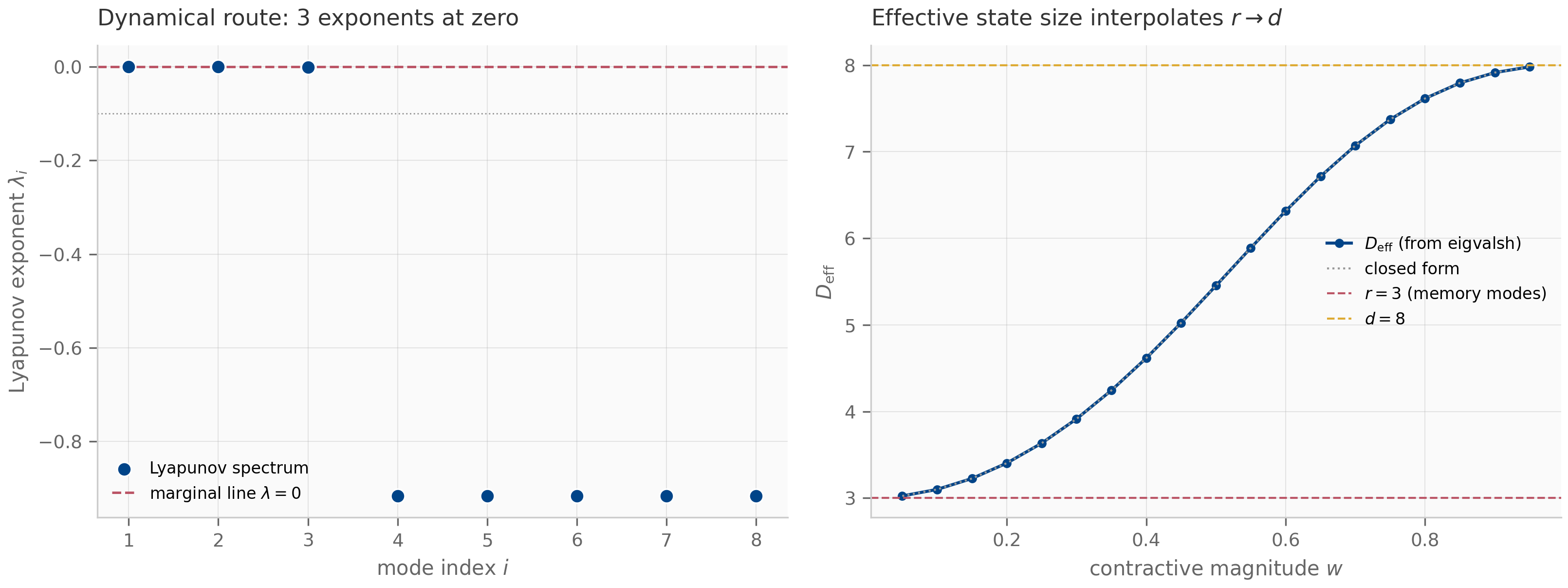
- (Two routes, one count.) The algebraic marginal count (from the eigenvalues) and the dynamical marginal count (from the Lyapunov spectrum) both equal for any slack separating the two levels. Independent computations — one algebraic, one dynamical — agree on the memory-mode count.
- (Effective state size.) With , the participation ratio is a continuous soft-count: as and as , interpolating between the marginal-mode count and the full dimension.
Part 1 is the anti-circularity guard that makes this a diagnostic rather than a tautology: an effective-dimension number “validated” by feeding it its own spectrum proves nothing, but two independent computations — the QR Lyapunov scan and the algebraic participation ratio — agreeing on a system whose is known by construction is real corroboration. The companion builds the system and confirms both routes return , with the measured participation ratio matching the closed form to ; the effective state size runs from at (nearly all memory in the marginal modes) to at (all eight modes comparably persistent).
Effective state size is the diagnostic complement to the capacity bound of §15.3: the bound says how many bits a -coordinate state could hold; the effective size says how many coordinates a particular system actually keeps alive. A model can satisfy the capacity bound with room to spare and still fail on long-range recall because, after training, its has collapsed to a handful of modes. Measuring that collapse on trained checkpoints — across training, across layers — is, again, B’s empirical program; an independent Julia implementation of the same QR-Lyapunov algorithm (matching the JAX spectra on shared anchors — the diagonal and DPLR closed-form values — to ) guards the numerics the program will lean on.
15.6 The mechanistic verdict
The impossibility theorems and the diagnostics meet in a mechanistic question: when a recurrent model underperforms a transformer on recall, what fails? The sharpest counter-evidence here comes from the architecture’s own side. Of Bick, Xing & Gu Bick et al. (2025) — the last author is Mamba’s creator — the Gather-and-Aggregate mechanism: a few attention heads do the heavy lifting of in-context retrieval (a “Gather” head extracts the relevant span, an “Aggregate” head integrates it), and recurrent models, lacking the sharp content-based addressing those heads provide, produce a smoother, lossier read. That the sharpest critique of recurrent recall comes from the architecture’s own side motivates the hybrids of Chapter 14 rather than abandoning the line. This is mechanistic evidence, not a theorem — we cite it, and offer Chapter 16’s outer-product reader as the analytic stand-in for the limitation, not a reproduction of the finding.
It also bears on why Chapter 14’s hybrids win: the recall gap that Lee et al. (2025) traces in Mamba–transformer hybrids is the same gap G&A localizes to a few heads. A handful of attention layers supply the sharp addressing the recurrence cannot, and the diagnostics of this chapter — Lyapunov spectrum, effective state size — are how you would find, in a trained hybrid, which layers carry the persistent memory and which have contracted to transients.
The assembled toolkit is three instruments: the capacity bound (an upper limit no fixed state escapes), the Lyapunov spectrum (is the state stable, and which modes persist), and the effective state size (how many modes actually do memory). Each is validated here against a system with a known answer. None is run on a trained network in this chapter — that boundary is deliberate. Probing trained SSMs and hybrids with these tools is pilot B’s contribution, and deciding what the prosecution’s file and the defense’s together imply for architecture choice is Chapter 17’s synthesis.
15.7 What’s next
Chapter 17 integrates the pilots: it takes the diagnostics built here and the benchmark protocol of Chapter 16 and turns them on the C1 (symplectic) and B (two-timescale) programs, weighing the counter-evidence of this chapter against the fourteen chapters of construction that precede it. The instruments of §§15.4–15.5 are exactly what B carries to trained checkpoints; the impossibility results of §15.2 are the ceiling against which Chapter 17 reads any empirical win. Looking back, this chapter closes the stability thread Chapter 13 opened: the matrix-memory spectrum that chapter computed at the architecture level (Proposition 13.1, Proposition 13.2) is now a quantity a diagnostic measures on a concrete, possibly trained, system.
15.8 Exercises
Exercise 15.1 (short)
A diagonal SSM carries complex modes, each stored at bits, over a vocabulary . Use Proposition 15.1 to give the longest sequence it can losslessly recall. Why is a real model’s usable length strictly smaller than ?
Solution
The state budget is bits, and each token costs bits, so . A real model recalls fewer than tokens because the counting bound assumes a lossless, injective encoding of prefixes into states; a trained recurrence instead superposes writes (interference, the Chapter 11 rank wall), uses finite arithmetic, and never reaches the information-theoretic optimum. The bound is the ceiling of the ceiling — necessary, far from sufficient.
Exercise 15.2 (short, code)
Run companions/ch15/jax/lyapunov_diagnostics.py. Report the per-mode scatter and
the mean-rate error for the non-normal ring. What do the two numbers together tell
you about trusting a Lyapunov diagnostic on a trained (hence non-normal) recurrence?
Solution
The ring’s per-mode error scatters by while the mean rate is exact to . Together they say: on a coupled, non-normal recurrence with near-degenerate moduli, an individual interior Lyapunov exponent is unreliable (the QR frame cannot isolate it), but the sum/mean — pinned by the divergence identity — is trustworthy. On a trained model, read the top exponent (stability) and the sum (total contraction) confidently; treat an interior exponent as reliable only when its modulus is well separated from its neighbors.
Exercise 15.3 (short, code)
From the same run, report the two marginal-mode counts (algebraic and dynamical) and the effective state size at and for the system. Why does reporting both counts matter?
Solution
Both counts return ; the effective state size is at and at . Reporting both routes matters because they are independent: the algebraic count comes from the eigenvalues, the dynamical count from the QR Lyapunov scan. Their agreement on a system whose is known by construction is what certifies the diagnostic is measuring a real property rather than re-reporting its own input — the anti-circularity guard. A single route, agreeing only with itself, could be measuring an artifact.
Exercise 15.4 (theory) — solution in §15.9
Prove Proposition 15.1. Model the recurrence’s post-prefix state as a function , argue every later output factors through , and apply the pigeonhole principle when . Then specialize to verbatim copy to obtain .
Exercise 15.5 (theory) — solution in §15.9
Prove part 2 of Proposition 15.2 (the divergence identity). Using one Benettin step with orthogonal, show , and conclude for every , independent of any mode-resolution.
Exercise 15.6 (theory) — solution in §15.9
Prove part 2 of Proposition 15.3. For the two-level spectrum ( modes at , at ), derive from the participation-ratio definition, and take the limits and .
15.9 Full solutions to theory exercises
Solution to Exercise 15.4
Fix the suffix that poses the queries; then for each prefix the model’s answers are a deterministic function of the state it holds after reading (the recurrence is deterministic, and everything downstream sees only through ). So the entire answer map factors as . If , then cannot be injective (pigeonhole): there exist with , so the model produces identical answers on and . The task requires different answers on and (they are in , distinguished by construction), so the model is wrong on at least one. For verbatim copy, is all length- strings (each must be reproduced, hence distinguished), so losslessness forces , i.e. .
Solution to Exercise 15.5
One Benettin step orthonormalizes the propagated frame: with orthogonal and upper-triangular with the sign convention . Take determinants: . Orthogonal matrices have , and , so
The Benettin estimate is , so summing over and exchanging the sums,
This holds for every and uses nothing about whether the individual have converged or whether modes are degenerate — the sum is exact even when the per-mode split is not.
Solution to Exercise 15.6
With , the two-level spectrum has entries with and entries with . Then
so by definition
As the contractive terms vanish: , the marginal-mode count. As every : , the full dimension. For it lies strictly between and , a continuous interpolation — the soft count of usable memory modes.
15.10 Companion code
The companions live in companions/ch15/{jax,torch,julia} and are float64
throughout; the JAX modules are canonical, the torch module mirrors the diagnostic
core with cross-framework parity pinned , and the Julia module is an
independent-language Lyapunov cross-check.
jax/copying_bound.py— the information-counting bound (Proposition 15.1): the state-capacity and lossless-requirement bits, the recall-cliff threshold, and the demonstration that Chapter 16’s slot model (imported, not re-implemented) cliffs exactly at . Producescopying-bound.png.jax/lyapunov_diagnostics.py— the Lyapunov estimator (Proposition 15.2) reusing Chapter 2’sqr_lyapunov, the constructed systems (DPLR from Chapter 13, selective/LTV from Chapter 9, an S4D-Lin-like degenerate system, and Chapter 2’s ring for the resolution limit), the divergence identity, and the regime/effective-state-size diagnostic with its two-route cross-check (Proposition 15.3). Produceslyapunov-validation.pngandregime-separation.png.torch/lyapunov_diagnostics.py— an eager mirror of the diagnostic core (QR Lyapunov, closed form, effective state size), pinned to the JAX outputs intorch/tests/test_ch15_torch.py; the instrument is framework-agnostic because pilot B runs it on trained torch models.julia/lyapunov_crosscheck.jl— a stdlib-only independent QR-Lyapunov and eigendecomposition, matching the JAX spectra (diagonal recovery, the DPLR closed form) and the effective-state-size closed form to .
PYTHONPATH=. python companions/ch15/jax/copying_bound.py
PYTHONPATH=. python companions/ch15/jax/lyapunov_diagnostics.py
make companion-jax-tests          # all chapters' JAX suites
make companion-torch-tests        # JAX↔torch parity
julia --project=companions/ch15/julia companions/ch15/julia/runtests.jl