Linear algebra for sequence models: structured matrices and conditioning

3.1 Eigenvalue decomposition and Jordan normal form

Chapter 1’s matrix exponential built directly on the spectral structure of $\statemat$. The fundamental theorem is:

A Jordan block of size $k$ for eigenvalue $\lambda$ looks like

i.e. eigenvalue on the diagonal, ones on the superdiagonal, zeros elsewhere. The matrix exponential of a Jordan block is

which is the source of the polynomial-in-$t$ factors mentioned in Chapter 1, §1.2 — they appear exactly when there are Jordan blocks of size $> 1$.

For SSM analysis, the diagonalizable case dominates. Almost every $\statemat$ arising from random initialization or from training is diagonalizable; the non-diagonalizable case is a codimension-one subset of parameter space and shows up only at carefully-tuned boundaries. In practice the assumption ”$\statemat$ is diagonalizable” is essentially always valid; the Jordan form is the worst-case fallback.

3.2 Singular value decomposition

The eigenvalue decomposition requires $\statemat$ to be square; for general (rectangular or possibly non-diagonalizable) matrices, the right tool is the singular value decomposition.

The SVD has three properties that make it the workhorse of numerical linear algebra:

1. It always exists. Unlike the eigenvalue decomposition, no diagonalizability or even squareness assumption is needed.
2. The singular values give the Frobenius and operator norms. $\norm{\statemat}_2 = \sigma_1$ (operator norm, equal to the largest singular value); $\norm{\statemat}_F = \sqrt{\sum_i \sigma_i^2}$.
3. It reveals low-rank structure cleanly. Truncating the SVD at rank $r < \rank(\statemat)$ — keeping only the top $r$ singular values and corresponding columns of $U, V$ — gives the best rank-$r$ approximation to $\statemat$ in both Frobenius and operator norms (the Eckart–Young theorem).

For square $\statemat$, the singular values are related to but distinct from the eigenvalues. The relationship $\sigma_i(\statemat)^2 = \lambda_i(\statemat^\top \statemat)$ (using descending order on both sides) lets you compute singular values via an eigenvalue problem on the Gram matrix $\statemat^\top \statemat$ — though in practice the QR-iteration-based SVD algorithm (LAPACK’s gesdd) is more numerically stable.

The SVD shows up explicitly in:

• Chapter 2’s Lyapunov-exponent computation (singular values of the propagated frame matrix).
• Chapter 8’s HiPPO matrix analysis (the conditioning of the projection operator is given by its SVD).
• Chapter 12’s delta-rule lineage (DeltaNet’s state update is a rank-1 SVD correction).

For a textbook treatment of the SVD’s properties and algorithms, Trefethen–Bau Trefethen & Bau (1997) Chapters 4–5 are the standard reference. Golub–Van Loan Golub & Van Loan (2013) covers the algorithmic details exhaustively.

3.3 Condition number

The condition number of a matrix $\statemat \in \R^{N \times N}$ (with respect to the operator norm) is

the ratio of the largest to smallest singular value (when $\statemat$ is invertible; otherwise $\kappa = \infty$). The condition number measures how much $\statemat$ amplifies relative input perturbations into relative output perturbations: if $\statemat \statevec = b$ and $b$ has relative error $\delta b / \norm{b}$, then the relative error in the computed solution can be as large as $\kappa(\statemat) \cdot \delta b / \norm{b}$.

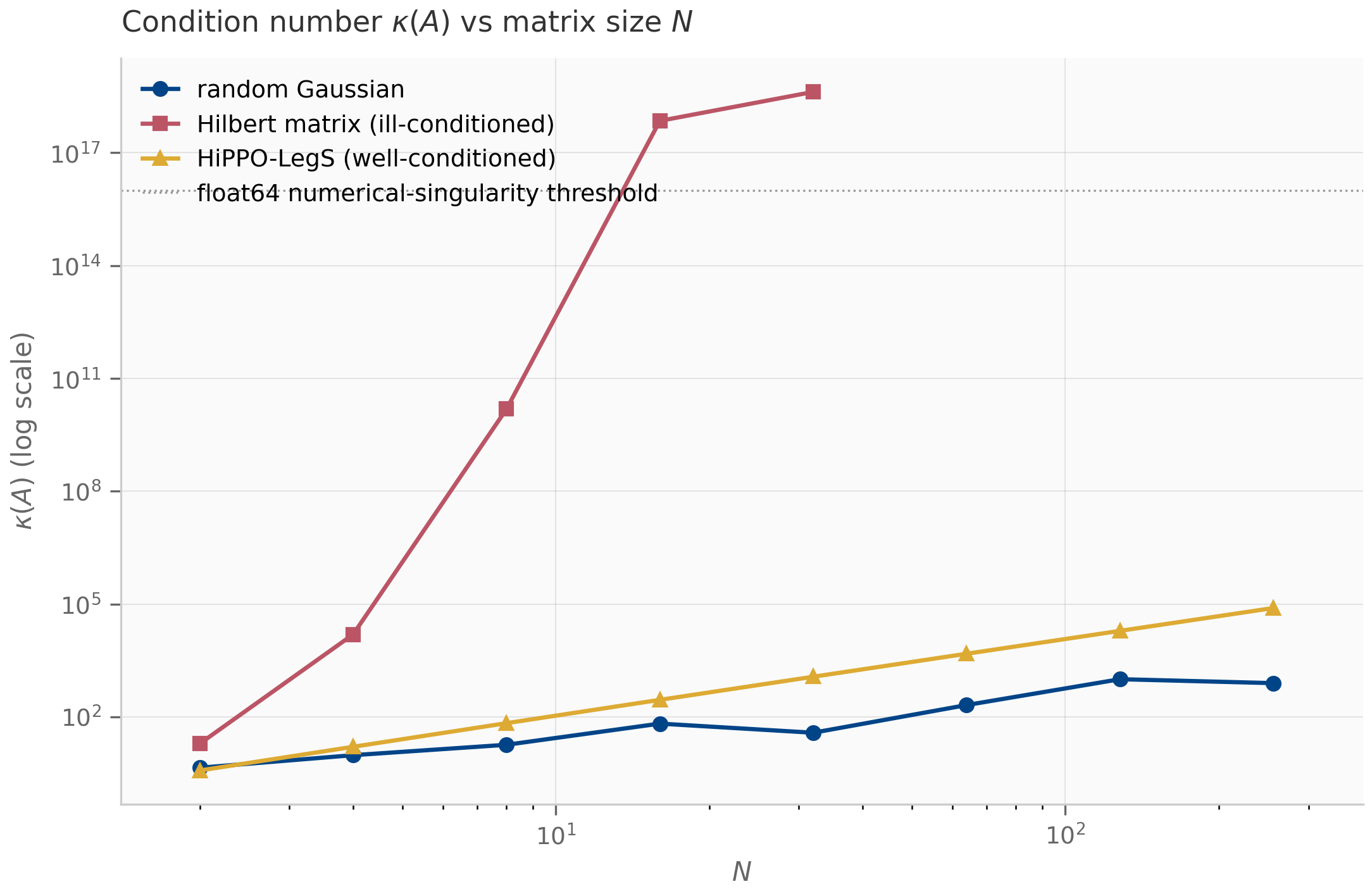
The qualitative scale: $\kappa = 1$ is the orthogonal case (no amplification); $\kappa \approx 10^k$ means losing roughly $k$ decimal digits of precision when solving a linear system. Double-precision floating point has about 16 decimal digits; matrices with $\kappa \gtrsim 10^{16}$ are numerically singular.

For SSMs, condition number matters in three places:

1. HiPPO matrix construction. The HiPPO-LegS matrix has structure that keeps its condition number bounded as $N$ grows — this is why HiPPO is the standard initialization. Random initializations typically give $\kappa$ growing as $N^{O(1)}$ or worse.
2. S4 kernel computation. S4’s Vandermonde-Cauchy kernel construction requires inverting a matrix with structured but potentially ill-conditioned columns. The paper carefully handles the conditioning; naive implementations don’t.
3. Mamba-3’s complex-state design. Chapter 10 discusses how Mamba-3 deliberately places eigenvalues in a region of the complex plane where the discrete-time map remains well-conditioned across the integration step.

3.4 Structured matrix families

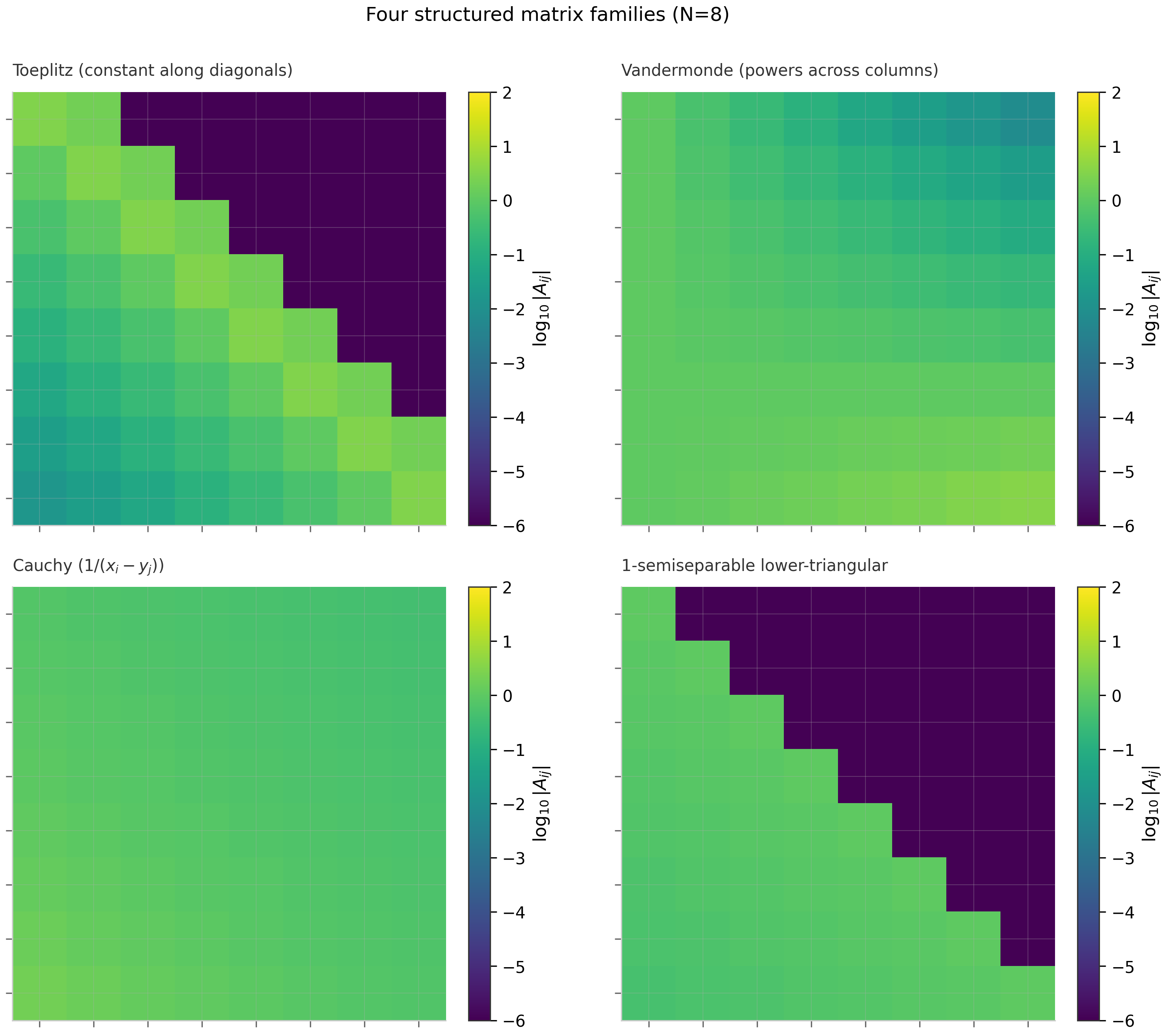
Four classes of structured matrices appear throughout the SSM literature. Each is parameterized by $O(N)$ numbers rather than the $O(N^2)$ a general matrix needs, and each admits fast matrix-vector products via specialized algorithms.

Toeplitz matrices

A Toeplitz matrix is constant along each diagonal:

Parameterized by $2n - 1$ values $(t_{-(n-1)}, \ldots, t_{n-1})$. Toeplitz matrices are the matrix form of convolutions: if $T$ is Toeplitz with first column $(t_0, t_1, \ldots, t_{n-1})$ and first row $(t_0, 0, \ldots, 0)$ (lower-triangular Toeplitz), then $T \statevec$ is the discrete convolution of the kernel $(t_0, t_1, \ldots)$ with $\statevec$. The FFT-based convolution algorithm computes $T \statevec$ in $O(n \log n)$ time.

LTI SSM convolutional view (Chapter 8) is exactly this: the operator that maps the input sequence $u$ to the output sequence $y$ via $y(t) = \int_0^t h(t-s) u(s) ds$ is a Toeplitz matrix at the discretization level, with first column equal to the discretized impulse response $h(0), h(\stepsize), h(2\stepsize), \ldots$.

Vandermonde matrices

A Vandermonde matrix has the form

parameterized by $n$ values $(x_1, \ldots, x_n)$. The defining property is that $(V \statevec)_i = \sum_{j=0}^{n-1} v_j x_i^j$ is a polynomial in $x_i$ evaluated at the node $x_i$. So Vandermonde matrices implement polynomial evaluation at $n$ points as a linear map.

Vandermonde matrices are notoriously ill-conditioned for nodes on the real line (condition number can grow exponentially), but well-behaved for nodes on the unit circle — which is why the FFT (Vandermonde with $x_i$ being roots of unity) is numerically stable.

The S4 kernel computation uses Vandermonde structure: evaluating $\sum_j c_j \lambda_j^k$ over $k = 0, 1, \ldots, L-1$ is exactly the Vandermonde-style polynomial evaluation. The S4 paper Gu et al. (2022) uses Cauchy-matrix tricks (next subsection) to make this evaluation stable.

Cauchy matrices

A Cauchy matrix has entries

parameterized by $n + m$ values $(x_1, \ldots, x_n, y_1, \ldots, y_m)$ with the $\{x_i\} \cap \{y_j\}$ empty (to avoid zero denominators). Cauchy matrices are dense — every entry depends on both indices — but the very structured dependence enables fast algorithms: a Cauchy matrix-vector product can be computed in $O(n \log^2 n)$ time using the fast multipole method.

Cauchy matrices appear in two places in the SSM literature: the S4 paper uses them as a numerically stable replacement for direct Vandermonde-style kernel evaluation, and the diagonal-plus-low-rank parametrization of $\statemat$ in S4 has a Cauchy-matrix interpretation when viewed through the partial-fraction decomposition of its transfer function.

Semiseparable matrices

A rank-$k$ semiseparable matrix has the property that every submatrix lying strictly above the main diagonal (and every submatrix lying strictly below) has rank at most $k$. Equivalently, the upper and lower triangular parts each have rank-$k$ structure.

The 1-semiseparable case — every off-diagonal block has rank at most 1 — is the structure exploited by Mamba-2’s SSD framework Dao & Gu (2024) . The 1-semiseparable lower-triangular matrix corresponding to a scalar-times-identity SSM is, explicitly,

where $a_i$ is the (scalar) recurrence coefficient at step $i$. The $(i, j)$ entry for $i > j$ is the product $a_{j+1} a_{j+2} \cdots a_i$. The SSD insight is that this matrix-vector product can be computed two ways: as a scan (the SSM view, $O(L)$ time) or as a structured matrix multiply (the attention view, $O(L^2)$ time but matmul-friendly on GPUs).

When $L$ is moderate (say $\le 8192$) and the GPU favors matmul over scan, the matrix view wins; when $L$ is huge, the scan view wins. Mamba-2’s chunked algorithm interpolates: matrix-multiplies within chunks of size $\sim 256$, scans across chunks. This is the structural reason Mamba-2 is faster than Mamba-1 on long sequences without sacrificing parallelism.

3.5 Low-rank corrections and rank-1 updates

A recurring pattern: take a structured matrix $S$ (diagonal, banded, or semiseparable) and add a small low-rank correction $U V^\top$ where $U, V \in \R^{n \times k}$ with $k \ll n$. The resulting matrix $S + U V^\top$ retains nearly the storage and matvec efficiency of $S$, and admits a closed-form inverse via the Sherman–Morrison–Woodbury identity:

The cost is dominated by inverting the $k \times k$ matrix $I + V^\top S^{-1} U$, not the $n \times n$ outer matrix.

This pattern appears in S4 explicitly: the HiPPO-LegS matrix isn’t diagonal, but it is “diagonal plus low-rank” — specifically, normal plus low-rank, which is what makes the kernel computation tractable. The S4 paper’s main algorithmic contribution is a specialized Sherman–Morrison-style trick for this exact decomposition.

The pattern recurs even more visibly in DeltaNet (Chapter 12), where the state update is

The middle factor is a rank-1 correction (specifically, an identity minus a rank-1 outer product), and the whole expression is one explicit-Euler step of an online gradient-descent update on the per-token association loss. The Longhorn paper Dao & Gu (2024) (well, the linear-attention lineage more generally) frames this as a discretization of an implicit-rank-1-correction online ODE.

The key takeaway: structured + low-rank corrections give you efficient matrix-vector products without giving up expressiveness. This is the design pattern unifying S4, DeltaNet, GLA, and the Mamba-2 SSD framework — each is a different choice of base structure and correction pattern.

3.6 Krylov subspaces: a primer

The Krylov subspace of order $k$ generated by a matrix $\statemat$ and a vector $b$ is

Krylov subspaces are the workhorse of iterative methods for large sparse linear systems: GMRES, conjugate gradient, Arnoldi iteration, Lanczos. All of them construct an orthonormal basis for $\mathcal{K}_k(\statemat, b)$ and solve a small ($k \times k$) projected problem instead of the original $n \times n$ one.

For SSMs, the Krylov picture is conceptual rather than algorithmic. The point is that $\mathcal{K}_k(\statemat, b)$ contains all the information the recurrence $\statevec_{t+1} = \statemat \statevec_t + \inputmat u_t$ can extract from the initial condition $b$ in $k$ steps. If the system has $n - k$ eigenvalues that are decoupled from the initial direction $b$ (the so-called “unreachable subspace”), the recurrence cannot recover them, and the effective dimension of the SSM is $k < n$. This is one rigorous reading of the Mamba copying-limitation results — the recurrence’s expressive ceiling is set by the Krylov dimension of $\statemat$ relative to the input.

A full treatment of Krylov methods would fill its own chapter; the curriculum revisits the picture in Chapter 8 (where the S4 kernel can be viewed as a structured Krylov-projection problem) and in Chapter 16’s empirical-methodology discussion of why some architectures can copy strings exponentially longer than others.

For a textbook coverage of Krylov-subspace methods, Trefethen–Bau Trefethen & Bau (1997) Chapters 32–40 give the full algorithmic treatment.

3.7 What’s next

You now have the linear-algebra vocabulary the rest of the book assumes. Chapter 4 picks up the discretization thread (started in Chapter 2, §2.4) and develops it systematically: order conditions, accuracy classes, the Butcher tableau, the bilinear and ZOH derivations in detail. Chapter 7 introduces the HiPPO theory that connects orthogonal-basis approximation theory to the $\statemat$ matrix structure of S4. Chapter 8 then shows how all four structured-matrix families combine in the S4 / S4D / S5 family.

If you’re impatient, Chapter 9’s Mamba-1/2/3 presentation is the payoff for the SSD discussion of §3.4 — the selective scan’s matmul-friendly chunkwise algorithm is exactly the 1-semiseparable matrix product algorithm.

3.8 Exercises

Six problems. Inline solutions for the shorter ones; full proofs for the theory exercises in §3.9.

Exercise 3.1 (computation)

Compute the Jordan normal form of $\statemat = \begin{pmatrix} 2 & 1 \\ 0 & 2 \end{pmatrix}$.

Exercise 3.2 (computation)

Compute the singular values of $\statemat = \begin{pmatrix} 3 & 0 \\ 0 & 4 \\ 0 & 0 \end{pmatrix}$ and its operator norm.

Exercise 3.3 (computation)

For the Vandermonde matrix with nodes $(x_1, x_2, x_3) = (1, 2, 3)$, write out the matrix and compute its determinant. Compare to the closed-form Vandermonde determinant $\det V = \prod_{i < j} (x_j - x_i)$.

Exercise 3.4 (computation)

Verify the Sherman–Morrison identity numerically: pick a random invertible $3 \times 3$ matrix $S$, vectors $u, v \in \R^3$, and check that $(S + u v^\top)^{-1}$ matches the closed-form expression to machine precision.

import numpy as np
rng = np.random.default_rng(0)
S = rng.standard_normal((3, 3))
u = rng.standard_normal(3)
v = rng.standard_normal(3)
direct = np.linalg.inv(S + np.outer(u, v))
S_inv = np.linalg.inv(S)
factor = 1.0 + v @ S_inv @ u
sherman = S_inv - np.outer(S_inv @ u, v @ S_inv) / factor
print(np.allclose(direct, sherman))  # True

Exercise 3.5 (theory) — solution in §3.9

Prove the Eckart–Young theorem: the best rank-$k$ approximation to a matrix $\statemat$ in the Frobenius norm is obtained by truncating its SVD at rank $k$. That is, if $\statemat = U \Sigma V^\top$ with singular values $\sigma_1 \ge \cdots \ge \sigma_n$, then $\statemat_k := \sum_{i \le k} \sigma_i u_i v_i^\top$ minimizes $\norm{\statemat - B}_F$ over all matrices $B$ of rank $\le k$.

Exercise 3.6 (theory) — solution in §3.9

Prove that a Toeplitz matrix $T \in \R^{n \times n}$ with $\norm{T \statevec}_2 \le C \norm{\statevec}_2$ for all $\statevec$ (operator-norm-bounded $T$) admits a matrix-vector product in $O(n \log n)$ time via the FFT. Specifically, show that any $n \times n$ Toeplitz $T$ can be embedded in a $2n \times 2n$ circulant matrix, whose matvec is exactly the FFT-IFFT pair applied to the kernel and input.

3.9 Full solutions to theory exercises

Solution to Exercise 3.5

The proof uses two ingredients: (a) the SVD’s unitary invariance of the Frobenius norm, and (b) the optimality of truncated diagonal matrices.

Setup. Let $\statemat = U \Sigma V^\top$ be the SVD with $\Sigma = \diag(\sigma_1, \ldots, \sigma_n)$ and $\sigma_1 \ge \cdots \ge \sigma_n \ge 0$. For any $B$ of rank $\le k$, write $B = U \widetilde B V^\top$ where $\widetilde B := U^\top B V$ also has rank $\le k$ (rank is invariant under invertible transformations). The Frobenius norm is invariant under orthogonal transformations:

So the problem reduces to: minimize $\norm{\Sigma - \widetilde B}_F$ over rank-$\le k$ matrices $\widetilde B$.

Diagonal reduction. Write $\widetilde B$ with its own SVD $\widetilde B = X D Y^\top$ where $D = \diag(d_1, \ldots, d_k, 0, \ldots, 0)$. Then

The middle trace term $\tr(\Sigma \widetilde B^\top) \le \sum_{i \le k} \sigma_i d_i$ by the von-Neumann trace inequality (with equality when $\widetilde B$‘s singular vectors align with $\Sigma$‘s — i.e. $\widetilde B$ is diagonal in the same basis as $\Sigma$). Optimizing $d_i$ to maximize this term subject to rank $\le k$ gives $d_i = \sigma_i$ for $i \le k$ and $d_i = 0$ for $i > k$, i.e. $\widetilde B = \diag(\sigma_1, \ldots, \sigma_k, 0, \ldots, 0)$.

Substituting back, the minimum value is $\norm{\Sigma - \widetilde B^*}_F^2 = \sum_{i > k} \sigma_i^2$, achieved by the truncated SVD $\statemat_k = U \diag(\sigma_1, \ldots, \sigma_k, 0, \ldots) V^\top = \sum_{i \le k} \sigma_i u_i v_i^\top$. ∎

(The proof for the operator norm follows the same structure but uses Weyl’s interlacing inequality instead of von-Neumann’s trace inequality; see Golub–Van Loan Golub & Van Loan (2013) for the detailed argument.)

Solution to Exercise 3.6

Let $T \in \R^{n \times n}$ be Toeplitz with entries $T_{ij} = t_{i-j}$ for some kernel $(t_{-(n-1)}, \ldots, t_{n-1})$.

Step 1 — Circulant embedding. Define a circulant matrix $C \in \R^{2n \times 2n}$ with first column

The first $n$ rows and first $n$ columns of $C$ exactly reproduce $T$ (the zero in the middle of $c$ is the “buffer” that prevents wrap-around contamination).

Step 2 — Padded matvec. Given $\statevec \in \R^n$, form $\widetilde \statevec = (\statevec, 0)^\top \in \R^{2n}$ (zero-padded). Then $(C \widetilde \statevec)_{1:n} = T \statevec$: the first $n$ entries of the circulant product are exactly the Toeplitz product, because the zero-padding ensures the wrap-around portion of the convolution doesn’t contaminate the top half.

Step 3 — Circulant matvec via FFT. Every $2n \times 2n$ circulant matrix $C$ is diagonalized by the discrete Fourier transform: $C = F^{-1} \diag(F c) F$, where $F$ is the $2n$-point DFT matrix. So

where $\odot$ is element-wise product. Both FFTs and the IFFT take $O(n \log n)$ time; the element-wise product is $O(n)$.

Total cost. $O(n \log n)$ for the FFTs + $O(n)$ for the element-wise multiply + $O(n)$ to extract the first $n$ entries = $O(n \log n)$. ∎

This is the exact algorithm used to compute LTI SSM convolutions in S4-family implementations: precompute the kernel $h(0), h(\stepsize), \ldots, h((L-1)\stepsize)$ once, then convolve with any input in $O(L \log L)$ time.

3.10 Companion code

Two runnable companions in companions/ch03/jax/:

• condition_number.py — plots κ(A) growth for random Gaussian, Hilbert, and HiPPO-LegS matrices as N grows; produces Figure 3.1
• structured_matrices.py — constructs Toeplitz / Vandermonde / Cauchy / 1-semiseparable matrices for N=8 and visualizes structural patterns; produces Figure 3.2

To run from the repo root:

PYTHONPATH=. python companions/ch03/jax/condition_number.py
PYTHONPATH=. python companions/ch03/jax/structured_matrices.py

Figures land in public/figures/ch03/.