LTI SSMs: S4, S4D, S5 as discretized continuous systems
The S4 architecture as a discretized HiPPO LTI system — the convolution–recurrence duality and its FFT kernel, the diagonal-plus-low-rank structure behind S4's fast kernel, S4D's diagonal restriction with by-construction stability, and S5's parallel associative scan.
On this page
- 8.1 State-space to discrete: the S4 setup
- 8.2 The structured state matrix, revisited
- 8.3 The convolution–recurrence duality
- 8.4 The Cauchy kernel: structure buys speed
- 8.5 S4D: the diagonal restriction
- 8.6 S5: the parallel associative scan
- 8.7 What’s next
- 8.8 Exercises
- Exercise 8.1 (computation)
- Exercise 8.2 (computation + code)
- Exercise 8.3 (code)
- Exercise 8.4 (theory) — solution in §8.9
- Exercise 8.5 (theory) — solution in §8.9
- Exercise 8.6 (theory) — solution in §8.9
- 8.9 Full solutions to theory exercises
- Solution to Exercise 8.4
- Solution to Exercise 8.5
- Solution to Exercise 8.6
- 8.10 Companion code
LTI SSMs: S4, S4D, S5 as discretized continuous systems
8.1 State-space to discrete: the S4 setup
Chapter 7 closed on a recurrence and called it the recurrent view of an S4-style layer. Make the layer explicit. S4 fixes a single-input, single-output (SISO) continuous system
with the HiPPO-LegS matrix of §7.3, , , and a scalar feedthrough. To run it on a sampled sequence we discretize at step . The S4 paper itself uses Chapter 4’s bilinear transform (§4.4), Gu et al. (2022) ; this book standardizes on the zero-order hold (§4.3) — the rule S5 Smith et al. (2023) and the Mamba line Gu & Dao (2024) later adopted, and one whose difference from bilinear the S4D ablations measure as negligible Gu et al. (2022) :
computed through the augmented matrix-exponential trick of §4.3 (the companion’s discretize_zoh stacks and exponentiates, sidestepping ).
What makes this an architecture rather than a fixed filter is which parts train. S4 learns , , and (the timescale, kept positive by the log), while are initialized from HiPPO and often frozen or updated slowly. Stability is inherited for free: by the §7.7 spectrum every eigenvalue of has negative real part, so Chapter 4’s ZOH proposition gives for every . The slowest mode (eigenvalue ) decays per step by — for the companion’s default that is , a long but strictly contracting memory.
This is one way to compute the layer. The rest of the chapter is, in large part, other ways to compute the same thing — and the surprising fact that they are equal.
8.2 The structured state matrix, revisited
Before the second view, recall why the HiPPO is special enough to deserve fast algorithms. It is dense and lower-triangular (§7.3), so a black-box and a black-box kernel would cost more than the structure warrants. The structure S4 exploits is that the HiPPO-LegS matrix is normal-plus-low-rank (NPLR): up to an orthogonal change of basis it is a normal matrix plus a rank-one correction, and after diagonalizing the normal part it becomes diagonal-plus-low-rank (DPLR),
with the (complex) diagonal of eigenvalues and a rank-one term Gu et al. (2022) . That the HiPPO-LegS matrix admits this diagonal-plus-rank-one form is not evident from the §7.3 closed form — it is a construction of the S4 paper, which we take as given rather than re-derive here. This is the same non-normality that §7.5 flagged as a conditioning hazard, now read constructively: the eigenvector basis is oblique (hence ill-conditioned), but the correction that makes non-normal is only rank one, and a rank-one correction is exactly what the Woodbury identity handles cheaply.
The DPLR form is the hinge for the rest of the chapter. Section 8.4 uses the full to compute S4’s kernel quickly; §8.5 throws away the term entirely and keeps only , which is S4D.
8.3 The convolution–recurrence duality
The recurrence of §8.1 is sequential: needs . Unrolling it from zero initial state exposes a second, fully parallel description. With ,
Define the SSM convolution kernel by . Then the output is a causal convolution plus the feedthrough:
(Convolution–recurrence duality.) For zero initial state, the SISO recurrence , produces exactly the convolution with kernel , . The recurrent form costs sequential steps; the convolution, computed by FFT, costs parallel work.
The proof (Exercise 8.4, §8.9) is the unrolling above made rigorous by induction. The two forms are not approximations of each other — they are the same numbers. The companion confirms it to machine precision: the recurrent lax.scan output and the FFT convolution agree to a measured residual in float64, which test_conv_recurrence_duality pins below .
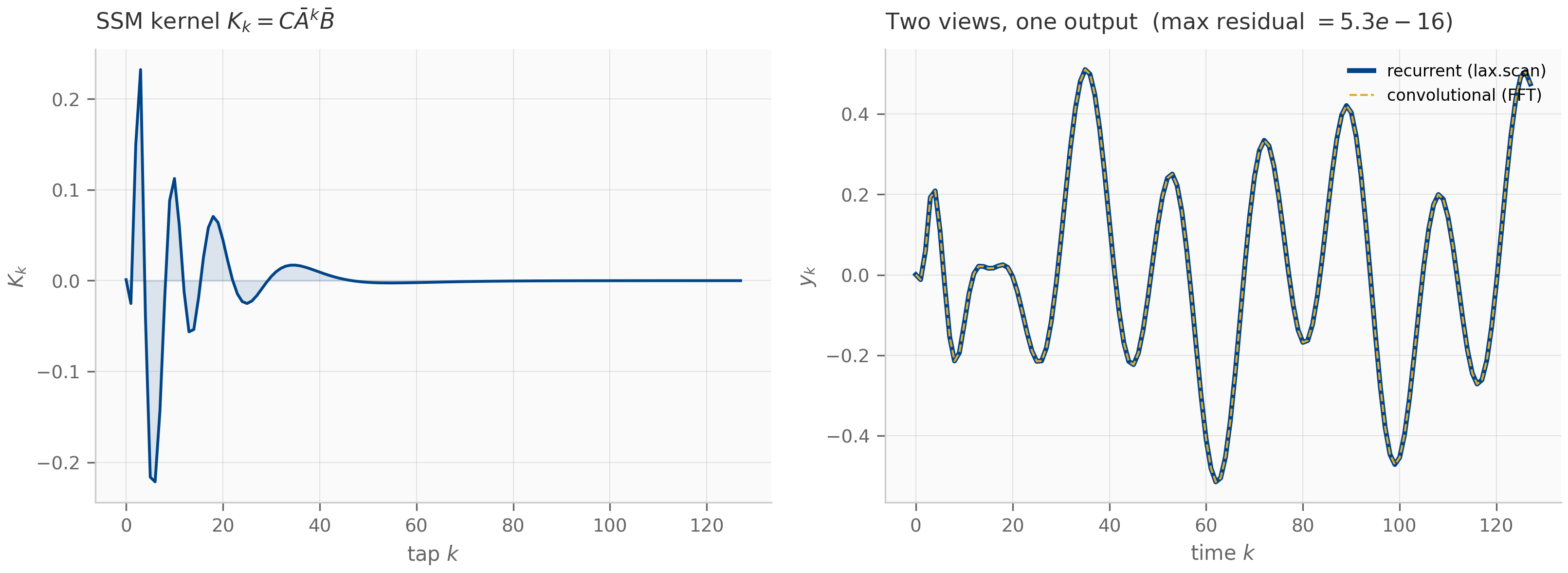
The duality is why S4 is practical: train as a convolution, deploy as a recurrence. Training sees whole sequences at once, so the parallel FFT wins; autoregressive inference produces one token at a time, so the scan with its state wins. One set of parameters, two runtimes.
8.4 The Cauchy kernel: structure buys speed
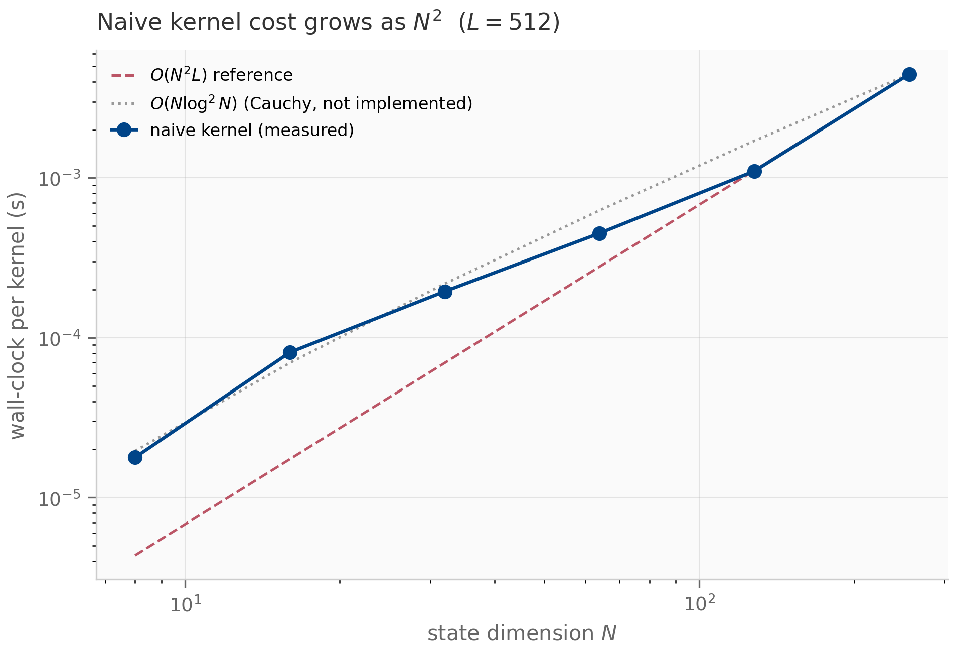
The duality leaves one cost open: building the kernel . Naively, iterates the state vector — one mat-vec per tap, in total. For the teaching regime that is exactly what the companion does, and it is plenty fast. S4’s published contribution is to compute the same kernel in near-linear time, , by using the DPLR structure of §8.2 Gu et al. (2022) .
The route is a generating function. Collect the taps into a polynomial and evaluate it on the unit circle: the truncated generating function is
a geometric series in the matrix . Recovering from evaluated at the -th roots of unity is one inverse FFT. The remaining cost is the resolvent , and here DPLR pays off: with built from the Woodbury identity turns the resolvent into a Cauchy matrix–vector product — entries — plus a rank-one correction. The whole kernel is then a Cauchy/Woodbury solve in plus the inverse FFT in (the §8.4 figure isolates the -scaling at fixed ); the dense never appears.
We present this kernel but do not implement it: the companions use the transparent naive kernel throughout (§8.10). The point of §8.4 is the shape of the cost, not the engineering — and the shape is what motivates S4D.
8.5 S4D: the diagonal restriction
The Cauchy machinery is the price of keeping the rank-one term . S4D asks what happens if we simply drop it Gu et al. (2022) — keep the diagonal , discard the low-rank correction. The state matrix is now genuinely diagonal, , and everything decouples mode by mode. The kernel collapses from a Cauchy computation to a Vandermonde sum:
with the per-mode diagonal ZOH input (this book’s convention; the S4D paper itself treats the integration rule as interchangeable — its base version keeps S4’s bilinear — and measures no noticeable difference between the two). In practice the real states are carried as complex conjugate pairs and the real kernel is reconstructed as .
(S4D Vandermonde kernel and stability.) For diagonal the kernel is the Vandermonde sum with . The discrete system is stable — every — if and only if for all .
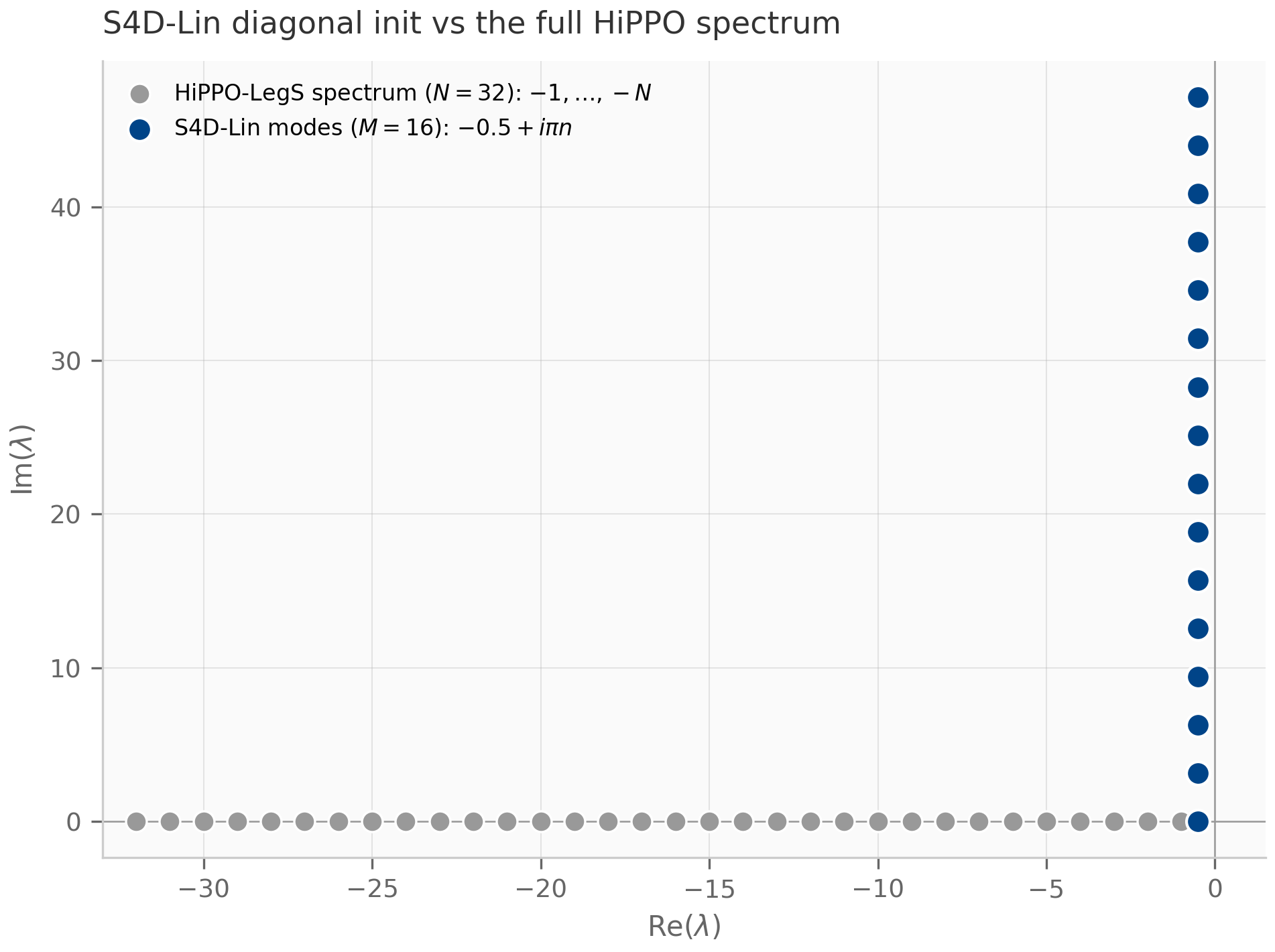
The derivation and the stability claim are Exercise 8.5 (§8.9). What makes S4D more than “S4 with worse expressivity” is how it secures the stability condition. The S4D-Lin initialization places the modes at , and — crucially — stores them in the parameterization
so that for any real value the parameters take. Stability is not hoped for; it is structural.
This is the constructive answer to the §7.5 conditioning hazard: where S4 must diagonalize an ill-conditioned non-normal matrix and hope the basis behaves, S4D never forms that basis at all — it parameterizes the eigenvalues directly and pins their real parts negative.
Diagonal state space models are not a downgrade in practice: with the right initialization they match full S4 on long-range benchmarks while being markedly simpler to implement Gupta et al. (2022) . The companion plots the S4D-Lin spectrum against the full HiPPO spectrum to make the restriction visible.
8.6 S5: the parallel associative scan
S4D made the state diagonal but still computed it as a convolution. S5 keeps the diagonal state and abandons the convolution for a parallel scan Smith et al. (2023) . Two changes. First, S5 is MIMO: one shared diagonal state of size drives input/output channels through and , instead of independent SISO systems. Second, it computes the recurrence
(diagonal , so is elementwise) with an associative scan. The trick is that a linear recurrence is an associative operation on pairs:
which composes “apply the first affine update, then the second.” Scanning over the pairs yields every state at once.
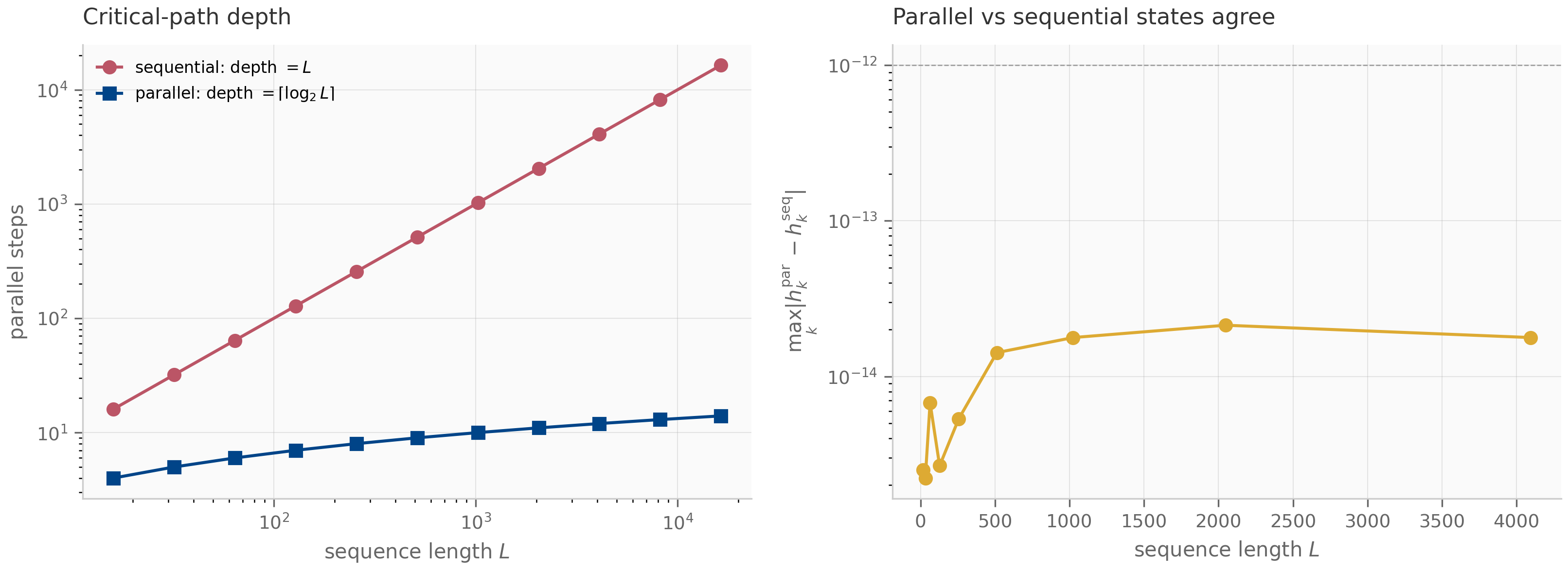
(Scan equivalence.) The operator above is associative, and the inclusive prefix scan of under has as its second components exactly the sequential states . A balanced reduction computes all prefixes in parallel depth Blelloch (1990) , versus the depth of the sequential recurrence.
The proof is Exercise 8.6 (§8.9). The companion pins the equivalence to machine precision — the associative scan and the sequential scan agree to about (pinned below ) — and contrasts the two on the algorithmic cost that actually differs: critical-path depth.
S5 deliberately stops at one diagonal SSM run in parallel. Its MIMO channel mixing and, above all, the move to input-dependent transitions are Chapter 9’s subject — and that move is what makes the associative scan indispensable rather than merely convenient.
8.7 What’s next
The thread of this chapter is that S4, S4D, and S5 are three computational treatments of one linear time-invariant system: a convolution and a recurrence that the duality proves equal (§8.3), a diagonal restriction whose stability is free (§8.5), and a parallel scan that reorders the same arithmetic into depth (§8.6). Time-invariance is what every one of these relies on — a fixed is what lets a single kernel exist and a single transition seed the scan.
Chapter 9 breaks time-invariance on purpose: Mamba makes functions of the input Gu & Dao (2024) (and the structured state-space duality Dao & Gu (2024) later reframes the result), which destroys the convolutional view and leaves the selective scan — the §8.6 primitive, now load-bearing — as the only way to compute the layer. Chapter 10 then replaces ZOH with the exponential-trapezoidal scheme of Chapter 4 when the selective dynamics turn stiff, in Mamba-3 Lahoti et al. (2026) ; that chapter is where the symplectic-integrator pilot finds its empirical anchor. Everything downstream inherits the discretized-LTI scaffold built here.
8.8 Exercises
Six problems mixing computation and theory. Short/numerical (8.1–8.3) have inline collapsible solutions; the theory exercises (8.4–8.6) have full worked solutions in §8.9.
Exercise 8.1 (computation)
Take a diagonal toy system , , , , and step . Compute and by the diagonal ZOH, then the first four kernel taps . Confirm the taps decay.
Solution
Diagonal ZOH acts mode-by-mode: and . So , and , . With the taps are :
Each tap is a sum of two decaying geometric sequences (rates and ), so the kernel decays monotonically — a discrete sum of exponentials, one per mode.
Exercise 8.2 (computation + code)
The S4D kernel sums one geometric sequence per mode. (a) Show that , so each mode decays at its own rate. (b) Show that a complex mode with weight and its conjugate with weight together contribute , explaining the real form. (c) Run companions/ch08/jax/s4d_kernel.py and confirm the Vandermonde kernel matches the recurrence oracle.
Solution
(a) , so and ; with this decays geometrically at rate per tap. (b) For any complex , since a number plus its conjugate is twice its real part; applying it with (and noting ) gives the claim. Carrying conjugate pairs and taking thus reproduces the -real-state kernel while storing only half as many complex numbers. (c) test_s4d_kernel_matches_recurrence_oracle pins the closed-form Vandermonde kernel against an independent complex-diagonal recurrence impulse response to .
Exercise 8.3 (code)
Run companions/ch08/jax/s4_duality.py and confirm the recurrent and convolutional outputs agree (the companion reports a residual below ). Then explain why the agreement would break if the FFT used length instead of .
Solution
The FFT computes a circular convolution of length equal to the transform size. With a length- transform, output position receives a contribution from kernel tap wrapped around the end of the sequence — a spurious term that the causal linear convolution does not contain, corrupting the early outputs. Zero-padding both signals to before the FFT makes the circular convolution agree with the causal linear one on the first positions (the wrapped terms land in the padded tail, which is discarded). The companion’s causal_conv_fft uses n = 2*L for exactly this reason; test_fft_pad_matches_direct_convolution pins the padded FFT against a direct convolution.
Exercise 8.4 (theory) — solution in §8.9
Prove the convolution–recurrence duality (Proposition, §8.3): for zero initial state, the SISO recurrence equals with .
Exercise 8.5 (theory) — solution in §8.9
Derive the S4D Vandermonde kernel from the diagonal recurrence, prove the discrete system is stable iff for all , and show that the S4D-Lin parameterization enforces stability for every parameter value.
Exercise 8.6 (theory) — solution in §8.9
Prove that the scan operator is associative, that its inclusive prefix scan reproduces the sequential states , and that a balanced reduction achieves parallel depth .
8.9 Full solutions to theory exercises
Solution to Exercise 8.4
Start from and . Claim: . Induct on . Base (): . Step: assuming ,
Now the output, using :
with . The sum is precisely the causal convolution , so . The lower-triangular Toeplitz structure of the map is the convolution.
Solution to Exercise 8.5
For diagonal the matrix exponential is diagonal, , and the ZOH input acts mode-by-mode: . The kernel inherits the diagonality,
a sum of geometric sequences — the Vandermonde form (the real version follows by pairing conjugates, Exercise 8.2). Stability: the kernel and the state stay bounded iff each geometric ratio satisfies . Since and , this holds iff for every . Finally, under S4D-Lin the real part is , and a negative exponential is strictly negative for every real exponent — so holds for all parameter values, with no constraint to enforce during training. Stability is built into the parameterization rather than maintained by it.
Solution to Exercise 8.6
Associativity. Write the action of a pair on a state as the affine map . Composition of affine maps is associative because function composition is. Concretely, with elementwise,
and the two right-hand sides are identical. Prefix scan reproduces the states. Let and be the inclusive scan. By induction the second component of equals : for it is (with ); and has second component . Depth. Because is associative, computing all prefixes is a prefix-sum problem, which a balanced binary reduction tree evaluates in sequential rounds with total work Blelloch (1990) — versus the rounds of the naive recurrence.
8.10 Companion code
Two language tracks for Chapter 8 — JAX (the reference, with the parallel scan) and PyTorch (the nn.Module operators). Julia is omitted here: the S4D reference and the associative-scan primitive both live in the JAX/PyTorch world, and a stdlib-Julia rebuild would add a third spelling without a third lesson. The JAX and torch companions are pinned bit-for-bit against each other, the cross-framework lesson Chapter 7 introduced.
JAX (companions/ch08/jax/):
s4_core.py— the harness-free S4 numerical core ported from the Week 4 source:make_hippo_legs,discretize_zoh/discretize_bilinear, the naive kernel, and the recurrent and convolutional views. The §8.3 duality lives here.s4_duality.py— emitskernel-duality.png(§8.3): kernel taps plus the two views overlaid.s4_kernel_cost.py— times the naive kernel across ; emitskernel-vs-n.png(§8.4).s4d_kernel.py— the S4D-Lin diagonal init and Vandermonde kernel (§8.5), complex128; emitss4d-spectrum.png.s5_scan.py— the S5 associative scan viajax.lax.associative_scan, with the sequential reference; emitss5-scan-depth.png(§8.6).tests/—test_s4.pypins the duality (recurrent convolutional), the kernel oracle, ZOH stability, and the FFT-pad guard;test_s4d_s5.pypins S4D by-construction stability, the Vandermonde-vs-recurrence cross-check, and S5 scan-equivalence.
PyTorch (companions/ch08/torch/):
s4d_kernel.py— the S4D kernel as annn.Module(fixed-init buffers), the Vandermonde computation ported from the reference S4D, in complex128.s5_sequential.py— the diagonal MIMO S5 as a sequential scan (PyTorch has no native parallel scan); the states match the JAX associative scan bit-for-bit.tests/test_s4d_torch.py— cross-framework parity: the torch S4D kernel and S5 states equal their JAX counterparts to within .
To run from the repo root:
# JAX (uses the uv .venv with jax, numpy, matplotlib)
PYTHONPATH=. python companions/ch08/jax/s4_duality.py
PYTHONPATH=. python companions/ch08/jax/s4_kernel_cost.py
PYTHONPATH=. python companions/ch08/jax/s4d_kernel.py
PYTHONPATH=. python companions/ch08/jax/s5_scan.py

# PyTorch (needs the .venv [torch] extra)
PYTHONPATH=. python companions/ch08/torch/s4d_kernel.py
PYTHONPATH=. python companions/ch08/torch/s5_sequential.py
All figures emit to public/figures/ch08/.